Almost ten years ago we published two tutorials on imputing missing data with the mice package (and a simpler walkthrough here). They are still among the most-read posts on this site, but the R ecosystem has moved on: random-forest imputation has become a default in machine-learning pipelines, and the old workhorses have faster successors.
Missing data is the daily reality of medical and epidemiological work: a patient skips a lab draw, a questionnaire item is left blank. So in this tutorial I use real health-survey data and compare three current imputation packages on it: mice (multiple imputation, still the reference method for statistical inference), missRanger (random-forest imputation, the fast successor of missForest), and VIM (k-nearest-neighbour imputation). Before any imputing I use naniar, the modern, ggplot-native toolkit for missing data, to picture where the gaps are. I also include the method most analyses actually use by default, dropping incomplete rows, because seeing why it fails is half the point.
I start from complete records, delete values myself, and check each package against the truth I hid.
library(NHANES)
library(mice)
library(missRanger)
library(VIM)
library(naniar) # ggplot-native missing-data visualisation
library(tidyverse)
library(broom) # tidy(): model estimates and CIs as a data frame
A complete dataset to work from
I use NHANES, the US National Health and Nutrition Examination Survey, which ships as an R package. The 2016 mice tutorial on this site used a simulated health dataset with age, cholesterol, blood pressure and BMI; here are the real versions of those variables. I keep adults, a handful of clinically sensible columns, and only the complete records, giving a ground-truth dataset with no missing values. To keep every package running in seconds I take a random 2,000 of them.
vars <- c(
  "Age",
  "Gender",
  "Height",
  "Weight",
  "BMI",
  "BPSysAve",
  "TotChol",
  "Diabetes",
  "Education"
)
set.seed(42)
nh <- NHANES |>
  filter(Age >= 20) |>
  select(all_of(vars)) |>
  drop_na() |>
  distinct() |>
  slice_sample(n = 2000) |>
  as.data.frame()
str(nh)
## 'data.frame':	2000 obs. of  9 variables:
##  $ Age      : int  50 57 69 49 26 30 59 33 53 80 ...
##  $ Gender   : Factor w/ 2 levels "female","male": 1 2 2 2 2 1 1 1 2 2 ...
##  $ Height   : num  164 169 172 163 185 ...
##  $ Weight   : num  75.8 70.8 91 67.7 82.7 ...
##  $ BMI      : num  28.1 24.7 30.8 25.4 24.1 ...
##  $ BPSysAve : int  133 113 122 123 107 122 141 104 126 103 ...
##  $ TotChol  : num  6.8 3.88 3.52 6.36 3.57 5.15 8.12 5.15 6.41 4.47 ...
##  $ Diabetes : Factor w/ 2 levels "No","Yes": 1 1 1 1 1 1 1 1 1 1 ...
##  $ Education: Factor w/ 5 levels "8th Grade","9 - 11th Grade",..: 3 2 5 1 5 3 3 5 3 4 ...
BPSysAve is average systolic blood pressure, TotChol is total cholesterol (mmol/L). A mix of numeric columns and factors (Gender, Diabetes, Education) is deliberate: imputing a category is a different problem than imputing a number, and a fair comparison should test both.
Deleting values the realistic way
Missing data comes in three flavors. MCAR (missing completely at random) means the missing values have nothing to do with anything: the easy case. MAR (missing at random) means the probability of a value being missing depends on other observed values. MNAR (missing not at random) means it depends on the missing value itself: the hard case no imputation fixes.
Health data is rarely MCAR: older participants miss more measurements, and that is a MAR pattern. So I make missingness in the clinical variables more likely with age, while age, sex, height and weight stay fully observed.
miss_vars <- c("BMI", "BPSysAve", "TotChol", "Diabetes", "Education")
ampute_mar <- function(data, seed) {
  set.seed(seed)
  p <- plogis(-2 + 0.9 * scale(data$Age)[, 1]) # older participant, more likely missing
  data |>
    mutate(across(all_of(miss_vars), (x) replace(x, runif(length(x)) < p, NA)))
}
amp <- ampute_mar(nh, 2026)
round(colMeans(is.na(amp)), 3)
##       Age    Gender    Height    Weight       BMI  BPSysAve   TotChol  Diabetes Education
##     0.000     0.000     0.000     0.000     0.152     0.152     0.160     0.147     0.155
That is about 15% missing in each clinical column, and only 996 of 2000 rows (50%) are still complete, so simply dropping incomplete rows would throw away the other 50% of the data. The missingness really is MAR: blood pressure is missing for 5% of the youngest third of participants but 29% of the oldest third. That age tilt is exactly what will bias a complete-case analysis later.
A first look with naniar
Before imputing anything, look at where the data is missing. The classic tool for this was VIM’s base-graphics aggr(), but naniar does the same job with ggplot2, so the plots match the rest of your analysis and theme like any other chart. Start with the share missing per variable. gg_miss_var() returns a plain ggplot, so I add the house theme straight onto it. (I define the theme here and reuse it for every figure below.)
dsp_colors <- c(
  "#0066CC",
  "#E8862D",
  "#159A6C",
  "#7D5BD6",
  "#D64580",
  "#2AA9B8",
  "#C9A227"
)
dsp_theme <- theme_minimal(base_size = 13) +
  theme(
    panel.background = element_rect(fill = "#F5F5F7", color = NA),
    panel.grid = element_line(color = "white"),
    axis.ticks = element_blank(),
    plot.title = element_text(face = "bold")
  )

gg_miss_var(amp) + dsp_theme + labs(title = "Share missing, by variable")
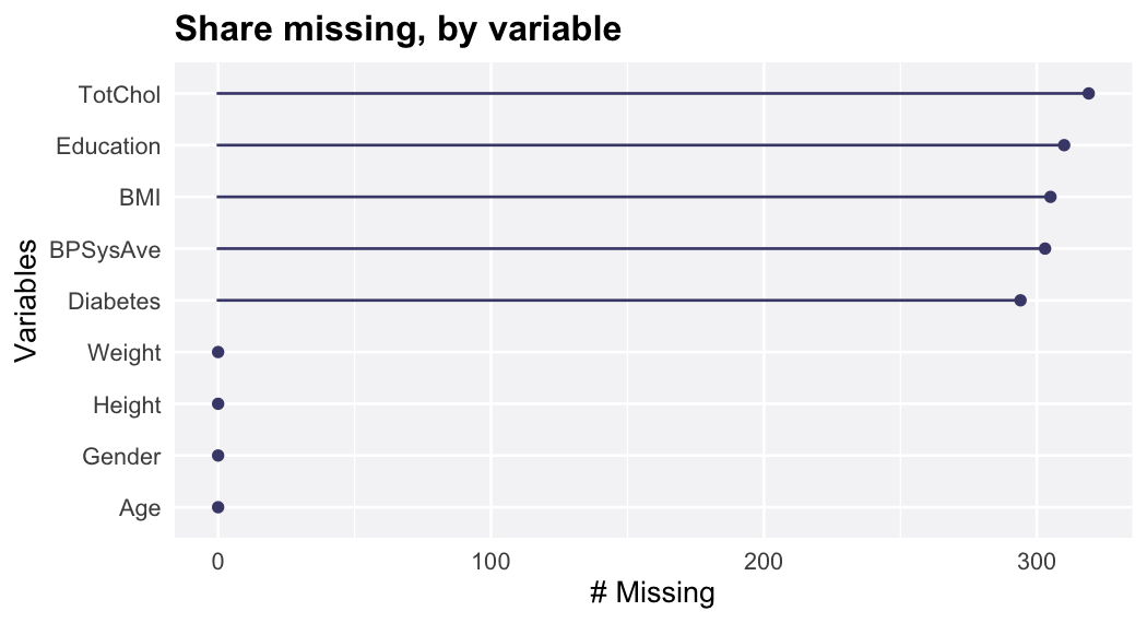
The five clinical variables are each ~15% missing while age, sex, height and weight are complete. But a per-variable count hides how the gaps line up across rows. vis_miss() draws the whole dataset, one row per participant with missing cells in dark, so you can see it directly.
vis_miss(amp, sort_miss = TRUE) +
  dsp_theme +
  theme(
    axis.text.x = element_text(angle = 30, hjust = 0),
    plot.margin = margin(t = 26, r = 40, b = 6, l = 6)
  )
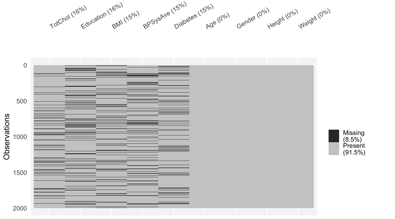
Most rows are missing something across those five columns, which is why dropping every incomplete row is so wasteful here. (naniar has more where these came from: gg_miss_upset() for the exact co-occurrence patterns, geom_miss_point() to show missing values on a scatter plot.)
Three ways to impute
mice builds a model for each incomplete variable from the others and cycles through them, m times with random draws, so you get m plausible complete datasets, not one. The defaults are sensible: predictive mean matching (pmm) for numbers, logistic and polytomous regression for factors.
imp_mice <- mice(amp, m = 5, printFlag = FALSE, seed = 1)
imp_mice$method
##       Age    Gender    Height    Weight       BMI  BPSysAve   TotChol  Diabetes Education
##        ""        ""        ""        ""     "pmm"     "pmm"     "pmm"  "logreg" "polyreg"
mice_list <- complete(imp_mice, "all") # a list of 5 completed datasets
missRanger iterates random forests over the incomplete variables (the missForest idea, rebuilt on the fast ranger engine). One call, one completed dataset.
imp_mr <- missRanger(amp, num.trees = 300, verbose = 0, seed = 1)
VIM’s kNN() fills each missing value from the k most similar participants, using a distance that handles numeric and categorical columns together.
imp_knn <- kNN(amp, k = 5, imp_var = FALSE)
On 2,000 rows mice (m = 5) took about a second, kNN about the same, and missRanger around three seconds. All three are fast here; on hundreds of thousands of rows missRanger’s ranger engine is the one built to scale.
Which package recovers the deleted values best?
Because I deleted the values myself, I can score each imputation against the truth. For the numeric columns I use NRMSE: root mean squared error on the deleted cells, divided by the variable’s standard deviation. Here is what that means, worked through on a small made-up example. Suppose I deleted the cholesterol reading (mmol/L) for five people, and compare the true values to what a package filled in:
| Person | True value | Imputed | Error | Error² |
|---|---|---|---|---|
| A | 5.0 | 4.6 | −0.4 | 0.16 |
| B | 6.2 | 6.0 | −0.2 | 0.04 |
| C | 4.5 | 5.3 | +0.8 | 0.64 |
| D | 7.0 | 6.5 | −0.5 | 0.25 |
| E | 5.3 | 5.1 | −0.2 | 0.04 |
RMSE (root mean squared error) is the typical size of those errors: square each one so a big miss counts more than a small one, average them, then take the square root, which here is √((0.16 + 0.04 + 0.64 + 0.25 + 0.04) / 5) ≈ 0.48 mmol/L. On its own that number means little: is 0.48 a big error for cholesterol? To make the score comparable across variables, I divide by the variable’s standard deviation, its natural spread. If cholesterol’s standard deviation is about 1.1, then NRMSE = 0.48 / 1.1 ≈ 0.43.
That scale is easy to read, because the standard deviation is roughly the error you would make by just filling every gap with the column mean. So NRMSE = 0 is perfect, NRMSE = 1 is no better than guessing the mean, and anything above 1 is worse than the mean, so the imputed values carry no real information. Our 0.43 means the errors are about 43% of the natural spread, so the imputation clearly beat guessing. For the factors (Diabetes, Education) there is no "spread" to divide by, so I simply score the share of categories the package got wrong. mice returns five datasets, so I average its five numeric imputations and take a majority vote for the factors, giving the fairest single estimate.
num_vars <- c("BMI", "BPSysAve", "TotChol")
cat_vars <- c("Diabetes", "Education")
score <- function(d) {
  map_dfr(c(num_vars, cat_vars), (v) {
    m <- is.na(amp[[v]])
    tibble(
      variable = v,
      value = if (v %in% num_vars) {
        sqrt(mean((d[[v]][m] - nh[[v]][m])^2)) / sd(nh[[v]])
      } else {
        mean(d[[v]][m] != nh[[v]][m])
      }
    )
  })
}

# mice gives 5 datasets: average the numbers, majority-vote the factors
mice_avg <- complete(imp_mice, "long") |> # the 5 datasets, stacked
  group_by(.id) |> # one group per row of `amp`
  summarise(
    across(all_of(num_vars), mean),
    across(all_of(cat_vars), (x) {
      factor(names(which.max(table(x))), levels = levels(x))
    })
  )

res <- bind_rows(
  mice = score(mice_avg),
  missRanger = score(imp_mr),
  kNN = score(imp_knn),
  .id = "package"
) |>
  mutate(
    package = factor(package, levels = c("mice", "missRanger", "kNN")),
    variable = factor(variable, levels = c(num_vars, cat_vars))
  )

res |>
  mutate(value = round(value, 3)) |>
  pivot_wider(names_from = variable, values_from = value)
## # A tibble: 3 × 6
##   package      BMI BPSysAve TotChol Diabetes Education
##   <fct>      <dbl>    <dbl>   <dbl>    <dbl>     <dbl>
## 1 mice       0.151     1.1    1.04     0.207     0.742
## 2 missRanger 0.339     1.03   0.951    0.18      0.719
## 3 kNN        0.827     1.07   1.09     0.214     0.748
acc <- res |>
  filter(variable %in% num_vars) |>
  mutate(variable = factor(variable, levels = rev(num_vars)))

ggplot(acc, aes(value, variable, color = package)) +
  geom_vline(xintercept = 1, linetype = 2, color = "#86868B") +
  geom_point(size = 3, position = position_dodge(width = 0.5)) +
  annotate(
    "text",
    x = 1,
    y = 0.55,
    label = "guessing the mean = 1",
    color = "#86868B",
    size = 3.4,
    hjust = 1.05
  ) +
  scale_color_manual(values = dsp_colors) +
  labs(
    title = "Recovery depends on the variable, not the package",
    subtitle = "NRMSE on the deleted cells. Lower is better.",
    x = "NRMSE",
    y = NULL,
    color = NULL
  ) +
  dsp_theme +
  theme(legend.position = "top")
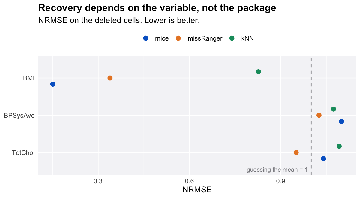
The surprise here is not which package wins; it is that the variable matters far more than the package. BMI is recovered almost perfectly (mice at 0.15 NRMSE), because height and weight are in the data and BMI is essentially a formula of them. Blood pressure and cholesterol are barely recoverable at all: every package lands near or above 1, meaning the imputed values are scarcely better than the column mean. That is not a failure of the software; it is the truth about the data. Systolic pressure and cholesterol are only weakly related to the other variables, so nothing can reconstruct an individual’s deleted reading. missRanger edges ahead on those noisy columns, mice on the near-deterministic BMI, but the honest headline is that no imputer manufactures information that was not there.
For Education the best method still misclassifies about 72% of the missing values, unsurprising for a five-level factor.
The analysis is where they differ
The usual reason to impute is to run a model on the completed data. Here is a standard epidemiological regression: systolic blood pressure on age, BMI, sex, diabetes and cholesterol. I fit it on the full data to get the truth, then refit it on the incomplete data four ways (dropping incomplete rows, mice, missRanger and kNN), then compare each one’s estimates and confidence intervals to that truth.
form <- BPSysAve ~ Age + BMI + Gender + Diabetes + TotChol
truth <- coef(lm(form, data = nh))
terms <- names(truth)[-1]
methods <- c("full data", "complete-case", "mice", "missRanger", "kNN")

lm_ci <- function(d) {
  # tidy estimate + 95% CI for every coefficient
  tidy(lm(form, data = d), conf.int = TRUE) |>
    filter(term %in% terms) |>
    transmute(term, est = estimate, lo = conf.low, hi = conf.high)
}

# mice pools across its 5 datasets (Rubin's rules); the rest are single fits
mice_pool <- summary(
  pool(with(imp_mice, lm(BPSysAve ~ Age + BMI + Gender + Diabetes + TotChol))),
  conf.int = TRUE
)

runs <- bind_rows(
  `full data` = lm_ci(nh),
  `complete-case` = lm_ci(amp),
  mice = mice_pool |>
    filter(term %in% terms) |>
    transmute(
      term = as.character(term),
      est = estimate,
      lo = `2.5 %`,
      hi = `97.5 %`
    ),
  missRanger = lm_ci(imp_mr),
  kNN = lm_ci(imp_knn),
  .id = "method"
) |>
  mutate(
    method = factor(method, levels = methods),
    term = factor(term, levels = terms)
  )
One plot shows both halves of the story at once. Each panel is one coefficient; each row is a method, with a dot for its estimate and a line for its 95% confidence interval. The dashed line is the full-data truth, and the top row is the full-data fit itself, the benchmark every method is trying to match.
tr <- tibble(term = factor(terms, levels = terms), truth = truth[terms])
term_lab <- c(
  Age = "Age (per year)",
  BMI = "BMI (per unit)",
  Gendermale = "Male vs female",
  DiabetesYes = "Diabetes: yes vs no",
  TotChol = "Cholesterol (per mmol/L)"
)

ggplot(runs, aes(est, method, color = method)) +
  geom_vline(
    data = tr,
    aes(xintercept = truth),
    linetype = 2,
    color = "#1D1D1F"
  ) +
  geom_pointrange(aes(xmin = lo, xmax = hi), size = 0.45) +
  facet_wrap(~term, scales = "free_x", labeller = labeller(term = term_lab)) +
  scale_y_discrete(limits = rev(methods)) +
  scale_color_manual(values = c("#1D1D1F", "#86868B", dsp_colors[1:3])) +
  labs(
    title = "Estimate and confidence interval, side by side",
    subtitle = "Dot = estimate, line = 95% CI. Dashed line = full-data truth; top row = the full-data fit.",
    x = "Estimate",
    y = NULL,
    color = NULL
  ) +
  dsp_theme +
  theme(legend.position = "none")
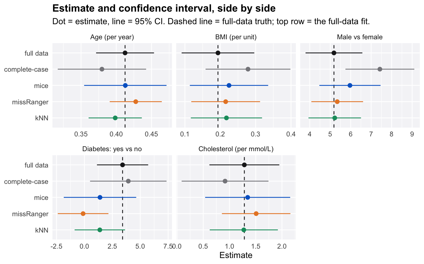
Read it in two passes. First the dots, the estimates. Dropping incomplete rows is the clear outlier: because missingness rises with age, the surviving rows skew younger and the estimates drift off the dashed line (the male-vs-female gap alone inflates from about 5 mmHg to around 7). All three imputers keep their dots close to the truth.
Now the lines, the confidence intervals. Deleting 15% of every clinical column can only lose information, so an honest interval should be at least as wide as the full-data one on top, never shorter. Yet missRanger’s and kNN’s lines come out shorter than the full data’s: single imputation treats every filled-in value as if it had really been measured, so the model believes it has more solid data than it does, and every standard error and p-value inherits that false confidence. Only mice widens its intervals (Rubin’s rules add the variation between its five imputations), the honest price of the missing data. It is the one method whose dot lands near the truth and whose line is honestly wide.
Summary
What to reach for:
- naniar: the first step of any imputation workflow.
gg_miss_var()andvis_miss()(plusgg_miss_upset()) show you where and how the data is missing, in plain ggplot2 that themes like the rest of your analysis. - missRanger: best point accuracy on the hard-to-predict columns, fast, one call. Use it when you need one completed dataset for prediction or a machine-learning pipeline, where honest standard errors are not the concern.
- mice: the only method here that carries imputation uncertainty into the model. Use it whenever the output is an estimate, a confidence interval, or a p-value, the typical medical or epidemiological analysis. Ten years on, it is still the right default for inference.
- VIM: its
kNN()is easy to reach for and handles mixed numeric/categorical data, but it trailed both other imputers here, so treat it as the fallback rather than the first choice.
And two lessons the NHANES data taught that a simulated dataset would have hidden. First, no imputer invents information: blood pressure and cholesterol were unrecoverable for every package, because they are only weakly related to the other variables. Second, dropping incomplete rows is the genuinely dangerous option under MAR: it biased the estimates while the imputers did not. The one thing none of this fixes is MNAR data, values missing because of the value itself, like high earners skipping the income question. There the honest move is a sensitivity analysis, not a better imputer.
That’s it. I hope you find this tutorial useful, and if you have questions, leave a comment below.

