NOAA analysts trace wildfire smoke plumes from satellite imagery every day and publish them as open GIS shapefiles. The files live at a predictable, date-based URL, so you can pull the current day’s smoke map straight into R and plot it over the U.S. in about 30 lines. We use sf to read the spatial data and ggplot2 to draw it.
The data source
The Hazard Mapping System (HMS), run by NOAA/NESDIS, is a daily analysis where operators trace smoke over North America from GOES satellite imagery. Each plume is a polygon with four attributes: the satellite, a start and end time, and a density class — Light, Medium, or Heavy. The daily shapefile is posted here:
.../Smoke_Polygons/Shapefile/YYYY/MM/hms_smokeYYYYMMDD.zip
Because the filename is just the date, we can build the URL programmatically and always get the latest map. Note that HMS finalizes a given day’s analysis the following morning (Eastern time), so today’s file may not exist until then — the robust helper at the end handles that.
Packages
library(sf)
library(dplyr)
library(ggplot2)
library(maps)
Get the data
We format the date into the URL, download and unzip the shapefile into a temp folder, and read it with st_read(). HMS names files by calendar date, so Sys.Date() gives us today’s map.
day <- Sys.Date()
ymd <- format(day, "%Y%m%d")
url <- sprintf(
  "https://satepsanone.nesdis.noaa.gov/pub/FIRE/web/HMS/Smoke_Polygons/Shapefile/%s/%s/hms_smoke%s.zip",
  format(day, "%Y"), format(day, "%m"), ymd)

zip <- file.path(tempdir(), basename(url))
dir <- file.path(tempdir(), paste0("hms_", ymd))
download.file(url, zip, mode = "wb", quiet = TRUE)
unzip(zip, exdir = dir)

smoke <- st_read(dir, quiet = TRUE)
Inspect what we got
Always look at the data before plotting it. st_read() returns an sf object — a data frame with a geometry column — so the usual tools work.
smoke                    # note the CRS line: WGS 84 / EPSG:4326
## Simple feature collection with 98 features and 4 fields
## Geometry type: POLYGON
## Dimension:     XY
## Bounding box:  xmin: -144.505 ymin: 12.23946 xmax: -11.87108 ymax: 85.46261
## Geodetic CRS:  WGS 84
## First 10 features:
##    Satellite        Start          End Density                       geometry
## 1  GOES-WEST 2026198 1200 2026198 1500   Light POLYGON ((-71.21715 19.0450...
## 2  GOES-WEST 2026198 1200 2026198 1500   Light POLYGON ((-71.99762 18.4664...
## 3  GOES-WEST 2026198 1200 2026198 1500   Light POLYGON ((-71.50895 18.6244...
## 4  GOES-WEST 2026198 1200 2026198 1500   Light POLYGON ((-76.61889 20.6635...
## 5  GOES-WEST 2026198 1200 2026198 1500   Light POLYGON ((-77.00836 21.2569...
## 6  GOES-WEST 2026198 1200 2026198 1500   Light POLYGON ((-80.49727 26.2337...
## 7  GOES-WEST 2026198 1200 2026198 1500   Light POLYGON ((-80.88491 26.4339...
## 8  GOES-WEST 2026198 1200 2026198 1500   Light POLYGON ((-82.60996 32.8358...
## 9  GOES-WEST 2026198 1200 2026198 1500   Light POLYGON ((-123.1322 42.0559...
## 10 GOES-WEST 2026198 1200 2026198 1500   Light POLYGON ((-103.8145 37.1463...
table(smoke$Density)     # how many plumes of each density today
##
##  Heavy  Light Medium
##     35     29     34
Two things to notice. First, the CRS is already EPSG:4326 (plain longitude/latitude), so no reprojection is needed. Second, Density takes three values — Light, Medium, Heavy — which is the variable we’ll color by. The Start/End fields use a YYYYDDD HHMM UTC format (day-of-year), but we won’t need them here.
Tidy the density classes
We coerce Density to an ordered factor and arrange() on it so heavy plumes are drawn last (on top of lighter ones), and call st_make_valid() because hand-drawn polygons occasionally self-intersect and would otherwise break the crop.
smoke <- smoke %>%
  filter(Density %in% c("Light", "Medium", "Heavy")) %>%
  mutate(Density = factor(Density, levels = c("Light", "Medium", "Heavy"))) %>%
  st_make_valid() %>%
  arrange(Density)
Map it
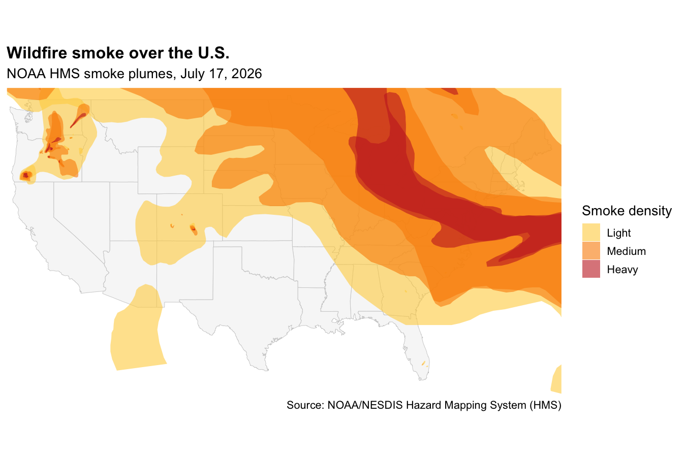
State outlines come from the maps package (pure CRAN, no API key). We crop the smoke to a lower-48 bounding box so the plot isn’t dominated by plumes over Canada and the oceans, then layer states underneath and smoke on top, colored by density.
states   <- st_as_sf(map("state", plot = FALSE, fill = TRUE))
bbox     <- st_bbox(c(xmin = -125, xmax = -66, ymin = 24, ymax = 50), crs = 4326)
smoke_us <- st_crop(smoke, bbox)

ggplot() +
  geom_sf(data = states, fill = "grey97", color = "grey80", linewidth = 0.2) +
  geom_sf(data = smoke_us, aes(fill = Density), color = NA, alpha = 0.6) +
  scale_fill_manual(values = c(Light = "#FFD24D", Medium = "#FB8C00", Heavy = "#C62828")) +
  coord_sf(xlim = c(-125, -66), ylim = c(24, 50), expand = FALSE) +
  labs(
    title    = "Wildfire smoke over the U.S.",
    subtitle = format(day, "NOAA HMS smoke plumes, %B %d, %Y"),
    fill     = "Smoke density",
    caption  = "Source: NOAA/NESDIS Hazard Mapping System (HMS)"
  ) +
  theme_minimal(base_size = 13) +
  theme(axis.text = element_blank(), panel.grid = element_blank(),
        plot.title = element_text(face = "bold"))
Reading the map
Today’s analysis has 98 smoke plumes over North America, 35 of them classed as heavy, and 57 intersecting the lower 48. The map turns that table into geography: where the polygons stack up and darken, smoke is thicker, and the plumes trace the path the smoke has travelled from its source fires — often hundreds of miles downwind. Re-run the code on a different day and both the numbers and the picture change; that is the point of building the URL from Sys.Date().
Because the counts and the map are generated from the same object, the paragraph above always describes the map you see — nothing is hard-coded.
A robust download
Run this early in the morning and today’s file may not be posted yet. This helper walks back day by day until it finds one that exists, so the script never dies on a missing date:
get_hms_smoke <- function(day = Sys.Date(), max_back = 3) {
  for (d in seq(0, max_back)) {
    date <- day - d
    ymd  <- format(date, "%Y%m%d")
    url  <- sprintf(
      "https://satepsanone.nesdis.noaa.gov/pub/FIRE/web/HMS/Smoke_Polygons/Shapefile/%s/%s/hms_smoke%s.zip",
      format(date, "%Y"), format(date, "%m"), ymd)
    zip <- file.path(tempdir(), basename(url))
    ok  <- tryCatch({ download.file(url, zip, mode = "wb", quiet = TRUE); TRUE },
                    error = function(e) FALSE)
    if (ok && file.exists(zip) && file.size(zip) > 0) {
      dir <- file.path(tempdir(), paste0("hms_", ymd))
      unzip(zip, exdir = dir)
      message("Using HMS smoke for ", date)
      return(st_read(dir, quiet = TRUE))
    }
  }
  stop("No HMS smoke file found in the last ", max_back, " days.")
}
Caveat: smoke aloft vs. smoke you breathe
HMS is a satellite product — it maps smoke seen from above, at any altitude. A thick plume on the map can sit five kilometers up and leave ground-level air clear, so HMS is a measure of smoke transport, not of what people are breathing. For surface air quality, pair it with ground PM2.5 from the EPA/USFS AirNow Fire and Smoke Map, which also has an API — a natural follow-up analysis.
That’s all. You now have a script that pulls a hand-analyzed satellite product and turns it into a national map, and re-runs itself for any day you like.


