Analyzing Google Trends Data in R

Google Trends shows the changes in the popularity of search terms over a given time (i.e., number of hits over time). It can be used to find search terms with growing or decreasing popularity or to review periodic variations from the past such as seasonality. Google Trends search data can be added to other analyses, manipulated and explored in more detail in R.

This post describes how you can use R to download data from Google Trends, and then include it in a chart or other analysis. We’ll discuss first how you can get overall (global) data on a search term (query), how to plot it as a simple line chart, and then how to can break the data down by geographical region. The first example I will look at is the rise and fall of the Blu-ray.

Analyzing Google Trends in R

I have never bought a Blu-ray disc and probably never will. In my world, technology moved from DVDs to streaming without the need for a high definition physical medium. I still see them in some shops, but it feels as though they are declining. Using Google Trends we can find out when interest in Blu-rays peaked.

The following R code retrieves the global search history since 2004 for Blu-ray.

library(gtrendsR)
library(reshape2)
  
google.trends = gtrends(c("blu-ray"), gprop = "web", time = "all")[[1]]
google.trends = dcast(google.trends, date ~ keyword + geo, value.var = "hits")
rownames(google.trends) = google.trends$date
google.trends$date = NULL

The first argument to the gtrends function is a list of up to 5 search terms. In this case, we have just one item. The second argument gprop is the medium searched on and can be any of web, news, images or youtube. The third argument time can be any of now 1-d, now 7-d, today 1-m, today 3-m, today 12-m, today+5-y or all (which means since 2004). A final possibility for time is to specify a custom date range e.g. 2010-12-31 2011-06-30.

Note that I am using gtrendsR version 1.9.9.0. This version improves upon the CRAN version 1.3.5 (as of August 2017) by not requiring a login. You may see a warning if your timezone is not set – this can be avoided by adding the following line of code:

Sys.setenv(TZ = "UTC")

After retrieving the data from Google Trends, I format it into a table with dates for the row names and search terms along the columns. The table below shows the result of running this code.

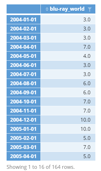
Plotting Google Trends data: Identifying seasonality and trends

Plotting the Google Trends data as an R chart we can draw two conclusions. First, interest peaked around the end of 2008. Second, there is a strong seasonal effect, with significant spikes around Christmas every year.

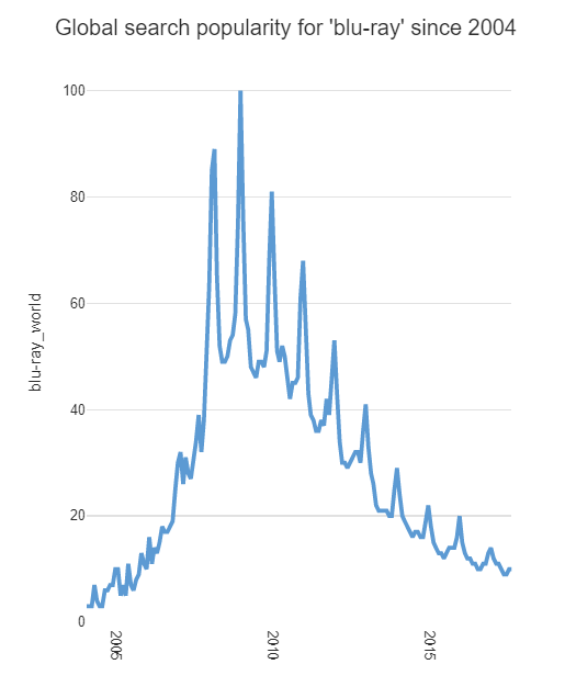
Note that results are relative to the total number of searches at each time point, with the maximum being 100. We cannot infer anything about the volume of Google searches. But we can say that as a proportion of all searches Blu-ray was about half as frequent in June 2008 compared to December 2008. An explanation about Google Trend methodology is here.

Google Trends by geographic region

Next, I will illustrate the use of country codes. To do so I will find the search history for skiing in Canada and New Zealand. I use the same code as previously, except modifying the gtrends line as below.

google.trends = gtrends(c("skiing"), geo = c("CA", "NZ"), gprop = "web", time = "2010-06-30 2017-06-30")[[1]]

The new argument to gtrends is geo, which allows the users to specify geographic codes to narrow the search region. The awkward part about geographical codes is that they are not always obvious. Country codes consist of two letters, for example, CA and NZ in this case. We could also use region codes such as US-CA for California. I find the easiest way to get these codes is to use this Wikipedia page.

An alternative way to find all the region-level codes for a given country is to use the following snippet of R code. In this case, it retrieves all the regions of Italy (IT).

library(gtrendsR)
geo.codes = sort(unique(countries[substr(countries$sub_code, 1, 2) == "IT", ]$sub_code))

Plotting the ski data below, we note the contrast between northern and southern hemisphere winters. It is also relatively more popular in Canada than New Zealand. The 2014 winter Olympics causes a notable spike in both countries but particularly Canada.

Create your own analysis

In this post I have shown how to import data from Google Trends using the R package gtrendsR. Anyone can click on this link to explore the examples used in this post or create your own analysis.