Panel data, along with cross-sectional and time series data, are the main data types that we encounter when working with regression analysis.
Types of data
- Cross-Sectional: Data collected at one particular point in time
- Time Series: Data collected across several time periods
- Panel Data: A mixture of both cross-sectional and time series data, i.e. collected at a particular point in time and across several time periods
When it comes to panel data, standard regression analysis often falls short in isolating fixed and random effects.
- Fixed Effects: Effects that are independent of random disturbances, e.g. observations independent of time.
- Random Effects: Effects that include random disturbances.
Let us see how we can use the plm library in R to account for fixed and random effects. There is a video tutorial link at the end of the post.
Panel Data: Fixed and Random Effects
For this tutorial, we are going to use a dataset of weekly internet usage in MB across 33 weeks across three different companies (A, B, and C). Find the dataset here: <a href="https://github.com/MGCodesandStats/datasets/blob/master/internetplm.csv.
Let us run our fixed (within) and random (random) effect models:
#Fixed Effects (within) and Random Effects (random)
library(plm)
plmwithin <- plm(usage~income+videohours+webpages+gender+age, data = mydata, model = "within")
plmrandom <- plm(usage~income+videohours+webpages+gender+age, data = mydata, model = "random")
summary(plmwithin)
Oneway (individual) effect Within Model
Call:
plm(formula = usage ~ income + videohours + webpages + gender +
    age, data = mydata, model = "within")

Balanced Panel: n=33, T=3, N=99

Residuals :
     Min.   1st Qu.    Median   3rd Qu.      Max.
-7001.684 -1744.973   -18.793  1212.604  6423.064

Coefficients :
              Estimate  Std. Error t-value  Pr(>|t|)
income         0.60389     0.14897  4.0538 0.0001451 ***
videohours  1261.43899   111.13253 11.3508 < 2.2e-16 ***
webpages      97.79839    42.06834  2.3248 0.0234299 *
gender     -1328.98316   812.05060 -1.6366 0.1068685
age           54.15710    36.54555  1.4819 0.1435128
---
Signif. codes:  0 ‘***’ 0.001 ‘**’ 0.01 ‘*’ 0.05 ‘.’ 0.1 ‘ ’ 1

Total Sum of Squares:    4312700000
Residual Sum of Squares: 692730000
R-Squared:      0.83937
Adj. R-Squared: 0.51719
F-statistic: 63.7531 on 5 and 61 DF, p-value: < 2.22e-16
summary(plmrandom)
Oneway (individual) effect Random Effect Model
   (Swamy-Arora's transformation)

Call:
plm(formula = usage ~ income + videohours + webpages + gender +
    age, data = mydata, model = "random")

Balanced Panel: n=33, T=3, N=99

Effects:
                   var  std.dev share
idiosyncratic 11356210     3370 0.912
individual     1093188     1046 0.088
theta:  0.1191

Residuals :
     Min.   1st Qu.    Median   3rd Qu.      Max.
-8153.757 -1808.112   -90.183  2101.833  8507.735

Coefficients :
               Estimate  Std. Error t-value  Pr(>|t|)
(Intercept) -1831.20613  1482.37880 -1.2353   0.21982
income          0.51416     0.12419  4.1401 7.627e-05 ***
videohours   1265.14090    94.06589 13.4495 < 2.2e-16 ***
webpages       95.35198    37.72137  2.5278   0.01316 *
gender      -1688.46458   708.69203 -2.3825   0.01923 *
age            57.27720    30.01488  1.9083   0.05944 .
---
Signif. codes:  0 ‘***’ 0.001 ‘**’ 0.01 ‘*’ 0.05 ‘.’ 0.1 ‘ ’ 1

Total Sum of Squares:    5790300000
Residual Sum of Squares: 1031900000
R-Squared:      0.82178
Adj. R-Squared: 0.77198
F-statistic: 85.7674 on 5 and 93 DF, p-value: < 2.22e-16
In the case of the first regression, we are accounting for fixed effects (or internet usage independent of time), while the second is accounting for random effects (including time).
Note that the variables gender and age which were deemed insigificant in the fixed effects regression are now being deemed significant in the random effects regression.
Analysing with fixef
Now, let us use fixef to isolate the effects of time on internet usage.
#Effect of time on internet usage
fixef(plmwithin,type="dmean")
         1          2          3          4          5          6          7          8          9         10         11
 3054.6050  -467.6298 -1557.9555   524.9491   -18.3859 -1374.6854  2300.6432  1890.2534  -541.1499  4721.5132   241.6241
        12         13         14         15         16         17         18         19         20         21         22
-1438.6650  2208.1437 -2036.5721  -848.0145   508.1098  -269.4162  2335.4139   803.8547 -3633.5643 -1399.4824  2142.2455
        23         24         25         26         27         28         29         30         31         32         33
  258.5465 -2458.9901 -1724.9200 -3979.0983    70.2551   717.6419  1289.9506 -1763.4756  2241.4846  2945.1578 -4742.3872
summary(fixef(plmwithin, type = "dmean"))
    Estimate Std. Error t-value Pr(>|t|)
1   3054.605   2860.669  1.0678  0.28561
2   -467.630   2452.521 -0.1907  0.84878
3  -1557.955   2368.244 -0.6579  0.51063
4    524.949   2734.229  0.1920  0.84775
5    -18.386   2861.050 -0.0064  0.99487
6  -1374.685   2719.298 -0.5055  0.61319
7   2300.643   2353.954  0.9774  0.32839
8   1890.253   2598.290  0.7275  0.46692
9   -541.150   2518.805 -0.2148  0.82989
10  4721.513   2619.317  1.8026  0.07146 .
11   241.624   2765.534  0.0874  0.93038
12 -1438.665   2868.905 -0.5015  0.61604
13  2208.144   2651.892  0.8327  0.40503
14 -2036.572   2549.967 -0.7987  0.42448
15  -848.015   2643.324 -0.3208  0.74835
16   508.110   2594.214  0.1959  0.84472
17  -269.416   2463.474 -0.1094  0.91291
18  2335.414   2662.246  0.8772  0.38036
19   803.855   2475.448  0.3247  0.74538
20 -3633.564   2504.424 -1.4509  0.14682
21 -1399.482   2727.735 -0.5131  0.60791
22  2142.245   2477.582  0.8647  0.38723
23   258.546   2702.259  0.0957  0.92378
24 -2458.990   3036.375 -0.8098  0.41803
25 -1724.920   2489.795 -0.6928  0.48844
26 -3979.098   2758.028 -1.4427  0.14910
27    70.255   2595.908  0.0271  0.97841
28   717.642   2494.345  0.2877  0.77357
29  1289.951   2575.964  0.5008  0.61654
30 -1763.476   2458.731 -0.7172  0.47323
31  2241.485   2441.171  0.9182  0.35851
32  2945.158   2725.083  1.0808  0.27980
33 -4742.387   2820.176 -1.6816  0.09265 .
---
Signif. codes:  0 ‘***’ 0.001 ‘**’ 0.01 ‘*’ 0.05 ‘.’ 0.1 ‘ ’ 1
Observe that weeks 10 and 33 are significant at the 10% level. For week 10, we see that usage across A, B, and C is higher than usual:

On the other hand, usage for week 33 across A, B, and C is lower than usual:

This could indicate that something is taking place across these particular weeks to cause internet usage to be higher and lower than usual. We see that using fixef has allowed us to isolate the effect of time in this regard.
Now, let us extract fixed effects – i.e. effects independent of time.
#Extracting fixed effects with fixef
twoway <-  plm(usage~income+videohours+webpages+gender+age+company,data=mydata,model="within",effect="time")
fixef(twoway,effect="time")
         a          b          c
 -451.3598 -1202.3393 -3451.6416
We see that of the three internet companies, company C has the largest negative coefficient.
Let’s subset usage for the three companies and see what is going on:
#Usage by provider
a <- subset(mydata, company=="a")
b <- subset(mydata, company=="b")
c <- subset(mydata, company=="c")
#Mean usage by provider
mean(a$usage)
mean(b$usage)
mean(c$usage)
[1] 11646.94
[1] 8851.848
[1] 6279.03
We see that mean internet usage for company C is lower than that of A and B.
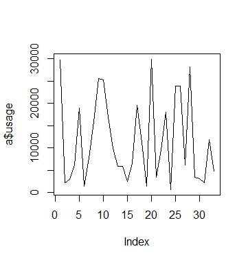
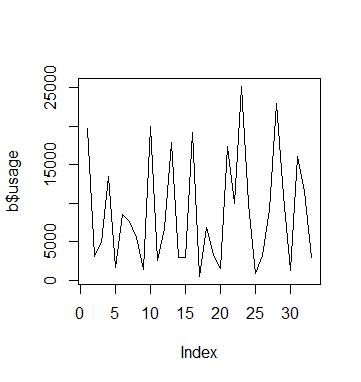
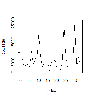
Moreover, visualising usage across the 33 weeks reveals an interesting insight:
#Usage visualisations
plot(a$usage,type='l')
plot(b$usage,type='l')
plot(c$usage,type='l')
We see that in the case of C, usage remains low overall but there are certain periods where we see a spike in usage. However, we see these spikes much more frequently for A and B.
In this regard, comparing fixed and random effects has allowed us to isolate the impact of time on usage patterns for C.
Conclusion
In this tutorial, you have learned:
- The difference between a fixed and random effects model
- How to use the plm library
- How to isolate fixed and random effects in a panel dataset
Many thanks for viewing this tutorial.


