In Part 1 of this series, we got started by looking at the ts object in R and how it represents time series data. In Part 2, I’ll discuss some of the many time series transformation functions that are available in R. This is by no means an exhaustive catalog. If you feel I left out anything important, please let me know. I compile these posts as a guide in RMarkdown which I plan to make available on the web soon.
Often in time series analysis and modeling, we will want to transform data. There are a number of different functions that can be used to transform time series data such as the difference, log, moving average, percent change, lag, or cumulative sum. These type of function are useful for both visualizing time series data and for modeling time series. For example, the moving average function can be used to more easily visualize a high-variance time series and is also a critical part the ARIMA family of models. Functions such as the difference, percent change, and log difference are helpful for making non-stationary data stationary.
Let’s start with a very common operation. To take a lag we use the lag() function from the stats package. It takes a ts object and a value for the lag argument.
tseries_lag1 <- lag(tseries, 1)
head(cbind(tseries, tseries_lag1))
tseries tseries_lag1
1999 Q4       NA      7.07667
2000 Q1  7.07667     10.38876
2000 Q2 10.38876     23.91096
2000 Q3 23.91096     14.49356
2000 Q4 14.49356     15.90501
2001 Q1 15.90501     28.00545
Notice that when we do this, tseries_lag1 is equivalent to tseries offset by 1, such that the value for 2000q1 in tseries become the value for 1999q4 in tseries_lag1 and so on. We can do this for any lag of our choosing. Let’s try 3 instead:
tseries_lag3 <- lag(tseries, 3)
head(cbind(tseries, tseries_lag3))
         tseries tseries_lag3
1999 Q2       NA      7.07667
1999 Q3       NA     10.38876
1999 Q4       NA     23.91096
2000 Q1  7.07667     14.49356
2000 Q2 10.38876     15.90501
2000 Q3 23.91096     28.00545
We can also do this in the opposite direction using a negative value for the lag argument, effectively creating a lead series instead:
tseries_lead1 <- lag(tseries, -1)
head(cbind(tseries, tseries_lead1))
         tseries tseries_lead1
2000 Q1  7.07667            NA
2000 Q2 10.38876       7.07667
2000 Q3 23.91096      10.38876
2000 Q4 14.49356      23.91096
2001 Q1 15.90501      14.49356
2001 Q2 28.00545      15.90501
Notice that tseries_lead1 now leads the original tseries by one time period.
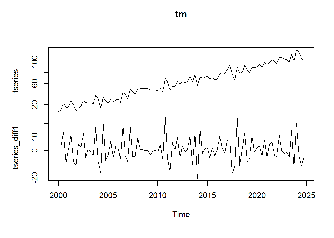
We can take differences of a time series as well. This is equivalent to taking the difference between each value and its previous value:
tseries_diff1 <- diff(tseries, lag = 1)
tm <- cbind(tseries, tseries_diff1)
head(tm)
tseries tseries_diff1
[1,]  7.07667            NA
[2,] 10.38876      3.312087
[3,] 23.91096     13.522201
[4,] 14.49356     -9.417399
[5,] 15.90501      1.411455
[6,] 28.00545     12.100441
plot.ts(tm)
As you can see, taking a difference is an effective way to remove a trend and make a time series stationary.
The difference can be calculated over more than one lag. To do so, simply alter the value of the lag argument.
tseries_diff2 <- diff(tseries, lag = 2)
tm <- cbind(tseries, tseries_diff2)
head(tm)
         tseries tseries_diff2
2000 Q1  7.07667            NA
2000 Q2 10.38876            NA
2000 Q3 23.91096     16.834288
2000 Q4 14.49356      4.104801
2001 Q1 15.90501     -8.005944
2001 Q2 28.00545     13.511896
plot(tm)
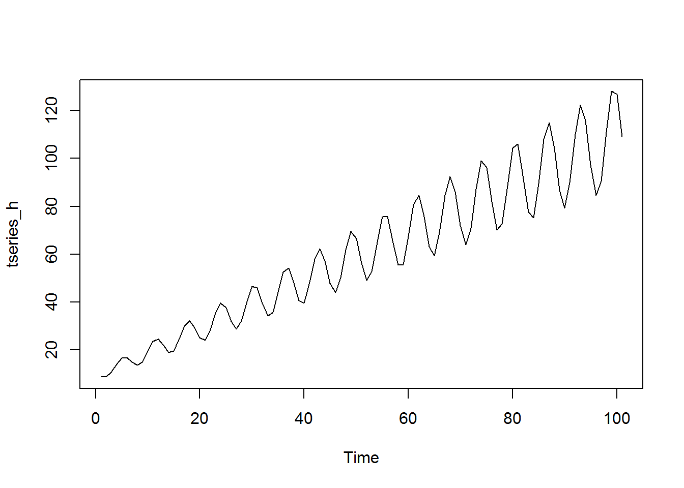
Some time series transformation functions are useful for series in which the variance gets larger over time. These range from the basic logarithm function to the Box-Cox group of transformations (of which the natural logarithm is a special case). We can take the log of a time series using the log function in the same way that we would take the log of a vector. Let’s generate a time series that has increasing variance:
trend <- ts(seq(from = 10, to = 110))
cycle <- ts(sin(trend)) * 0.2 * trend
tseries_h <- trend + cycle
plot.ts(tseries_h)
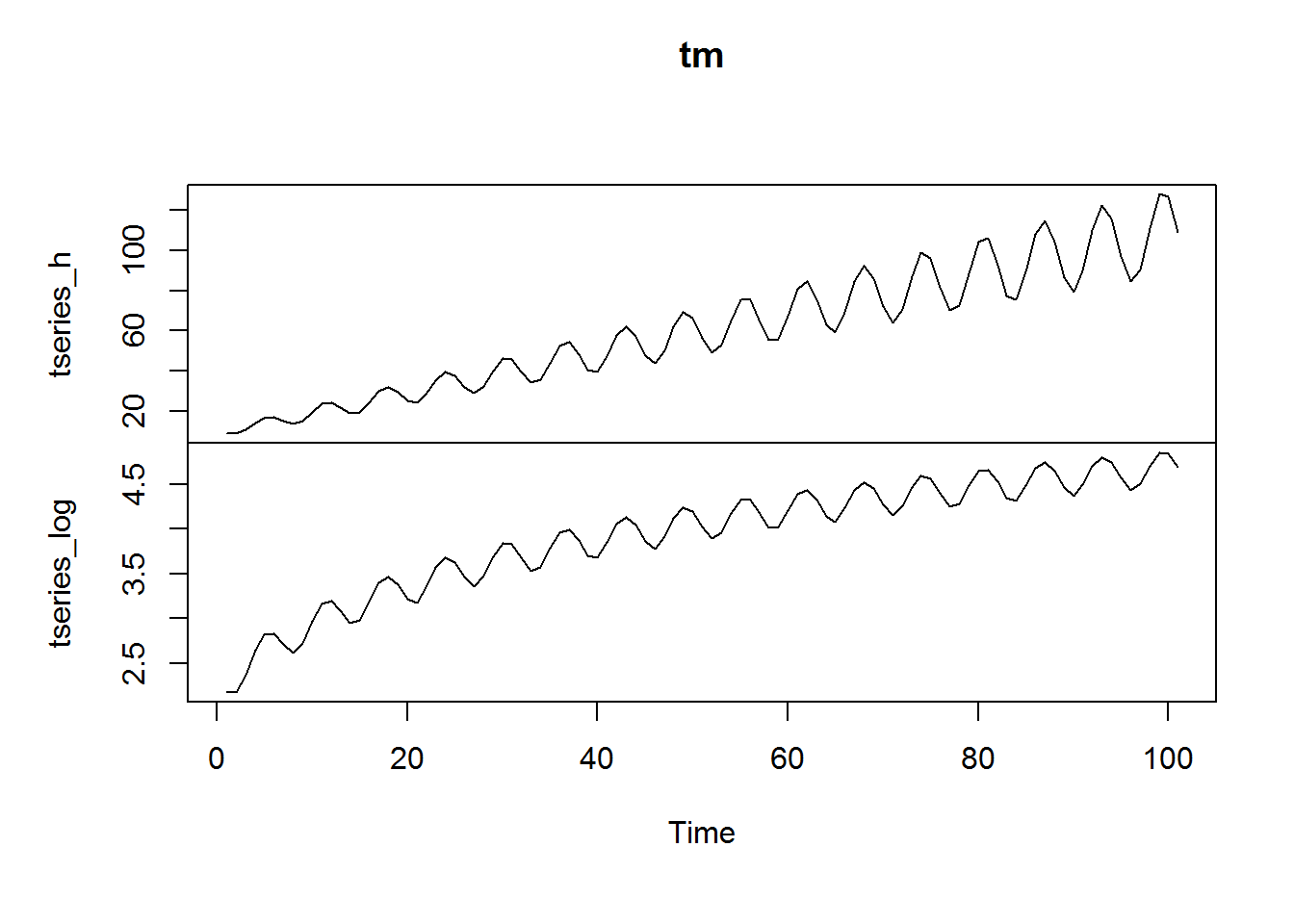
As we’ll discuss in more detail, the prevalence of increasing, or more generally non-constant, variance is called heteroskedasticity and can cause problems in linear regression. Often, it will need to be corrected before modeling. One way to do this is taking a log:
tseries_log <- log(tseries_h)
tm <-cbind(tseries_h, tseries_log)
plot.ts(tm)
There are other more advanced ways of eliminating non-constant variance, one of which is the Box-Cox transformation, which allows us a bit more control over the transformation. The Box-Cox takes the form (Hyndman and Athanasopoulos, 2013):
$$w_t = \begin{cases} \log{ y_t }, \text{ if } \lambda = 0; \\ \frac{ ({y_t}^{\lambda} – 1) }{ \lambda },\text{ otherwise } \\ \end{cases} $$
In order to demonstrate the Box-Cox transformation, I’ll introduce Rob Hyndman’s `forecast` package:
library(forecast)
It has two functions that are of use here. The primary function is BoxCox(), which will return a transformed time series given a time series and a value for the parameter lambda:
plot.ts(BoxCox(tseries_h, lambda = 0.5))
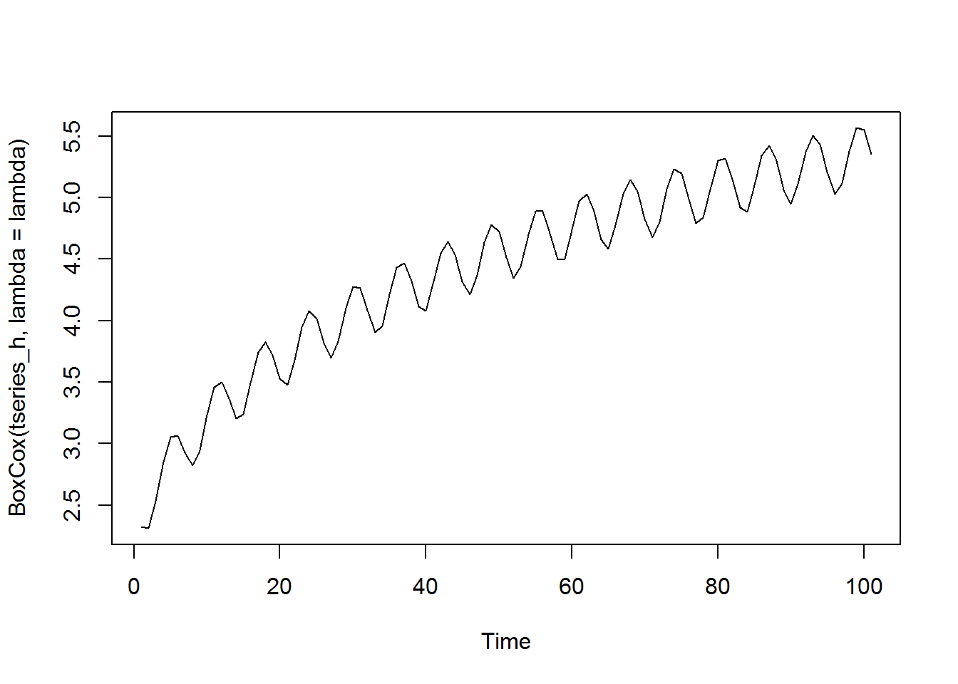
Notice that this value of lambda here does not entirely take care of the heteroskedasticity problem. We can experiment with different values of lambda, or we can use the BoxCox.lambda() function, which will provide us an optimal value for parameter lambda:
lambda <- BoxCox.lambda(tseries_h)
print(lambda)
[1] 0.05527724
plot.ts(BoxCox(tseries_h, lambda = lambda))
The BoxCox.lambda() function has chosen the value 0.055. If we then use this value in our BoxCox() function, it returns a time series that appears to have constant variance.
Another common calculation that we may want to perform on time series is the percent change from one period to another. Because it seems that R does not have a function for performing this calculation, we can do it ourselves.
tseries_pch <- tseries / lag(tseries, -1) - 1
head(cbind(tseries, tseries_pch))
         tseries tseries_pch
2000 Q1  7.07667          NA
2000 Q2 10.38876  0.46802901
2000 Q3 23.91096  1.30161865
2000 Q4 14.49356 -0.39385287
2001 Q1 15.90501  0.09738501
2001 Q2 28.00545  0.76079409
We can turn this into a function so that we can easily calculate percent change in the future. We’ll add an argument to specify the number of periods over which we want to calculate the change and set it to 1 by default. Additionally, we’ll add some argument verification.
pch <- function(data, lag = 1) {
    # argument verification
    if (!is.ts(data)) stop("data must be of type ts")
    if (!is.numeric(lag)) stop("lag must be of type numeric")
    # return percent change
    data / lag(data, -lag) - 1
}
head(cbind(tseries, pch(tseries)))
         tseries pch(tseries)
2000 Q1  7.07667           NA
2000 Q2 10.38876   0.46802901
2000 Q3 23.91096   1.30161865
2000 Q4 14.49356  -0.39385287
2001 Q1 15.90501   0.09738501
2001 Q2 28.00545   0.76079409
Now if we wished to calculate the percentage change over more than one period we can do so. Let’s say we wanted to calculate the year over year percent change. We can call our pch() function with a lag of 4.
tseries_pchya <- pch(tseries, lag=4)
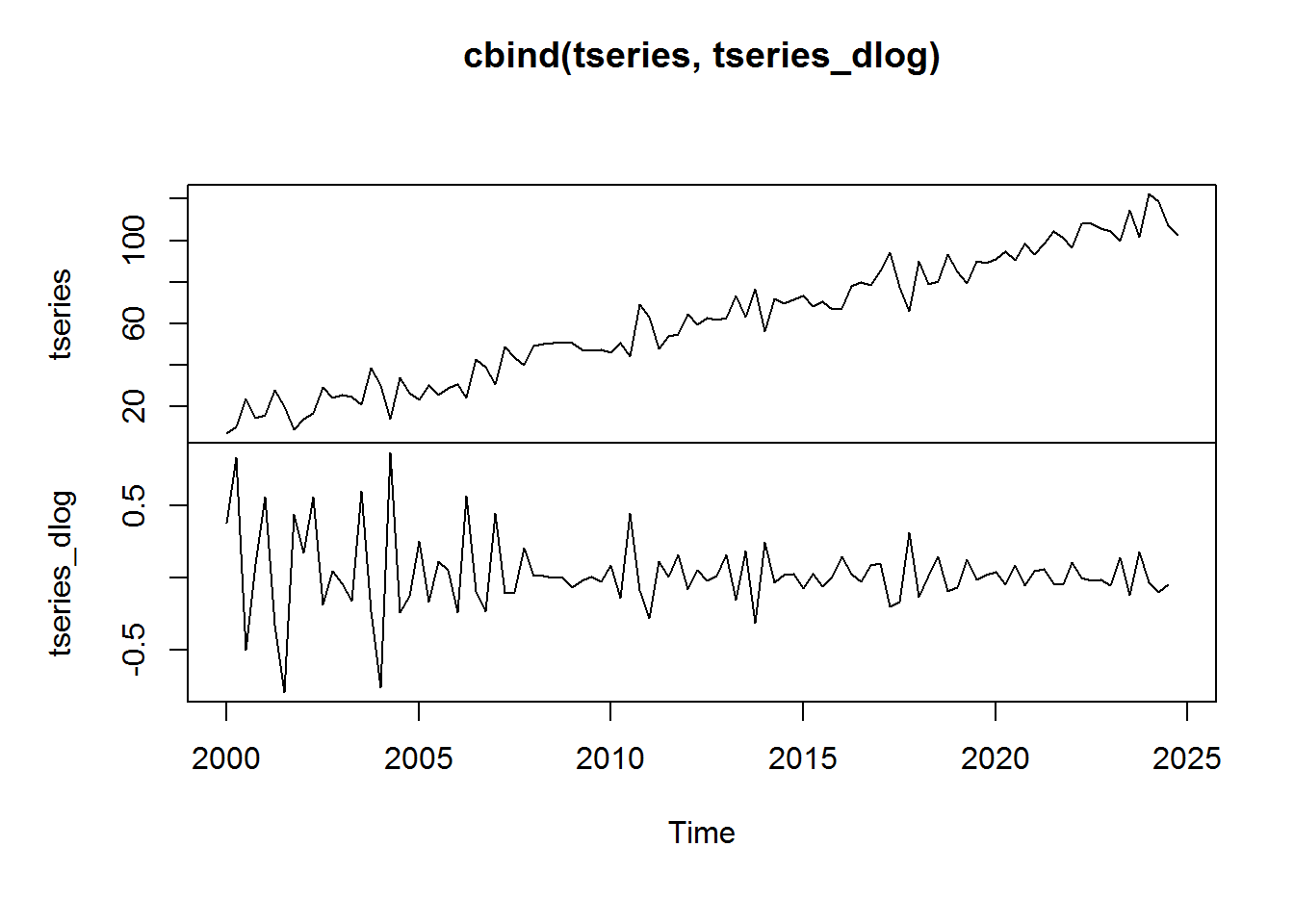
Two of the functions that we have discussed so far, the difference and the log, are often combined in time series analysis. The log difference function is useful for making non-stationary data stationary and has some other useful properties. We can calculate the log difference in R by simply combining the log() and diff() functions.
tseries_dlog <- ts(diff(log(tseries)), start = c(2000, 1), frequency = 4)
plot.ts(cbind(tseries, tseries_dlog))
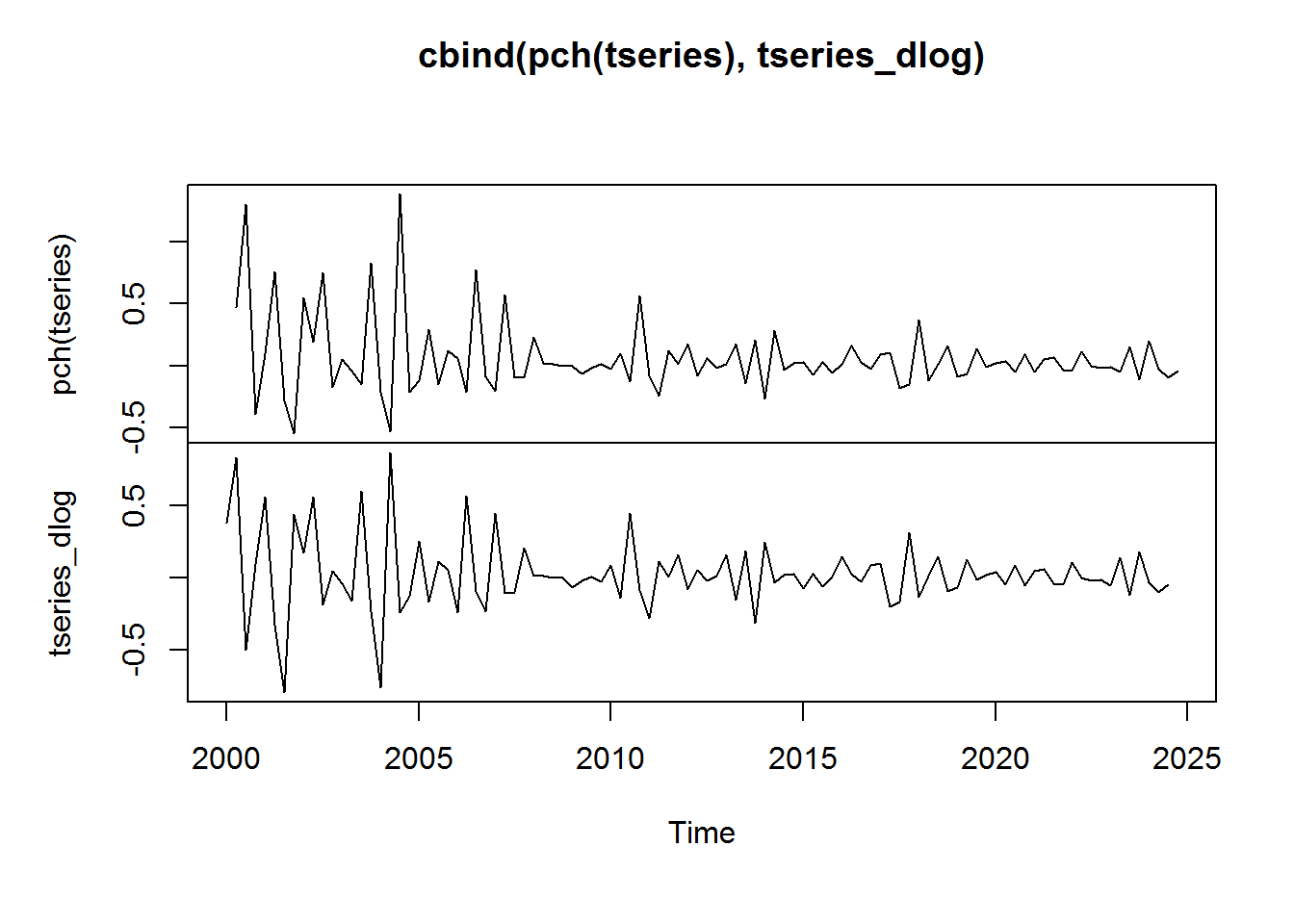
Notice that after taking the log return, tseries appears to be stationary. We see some higher than normal volatility in the beginning of the series. This is due largely to the fact that the series levels start off so small. This leads into a nice property of the log return function, which is that it is a close approximation to the percent change:
plot.ts(cbind(pch(tseries), tseries_dlog))
This similarity is only approximate. The relationship does break down somewhat when the percent change from one period to the next is particularly large. You can read a good discussion of this topic here.
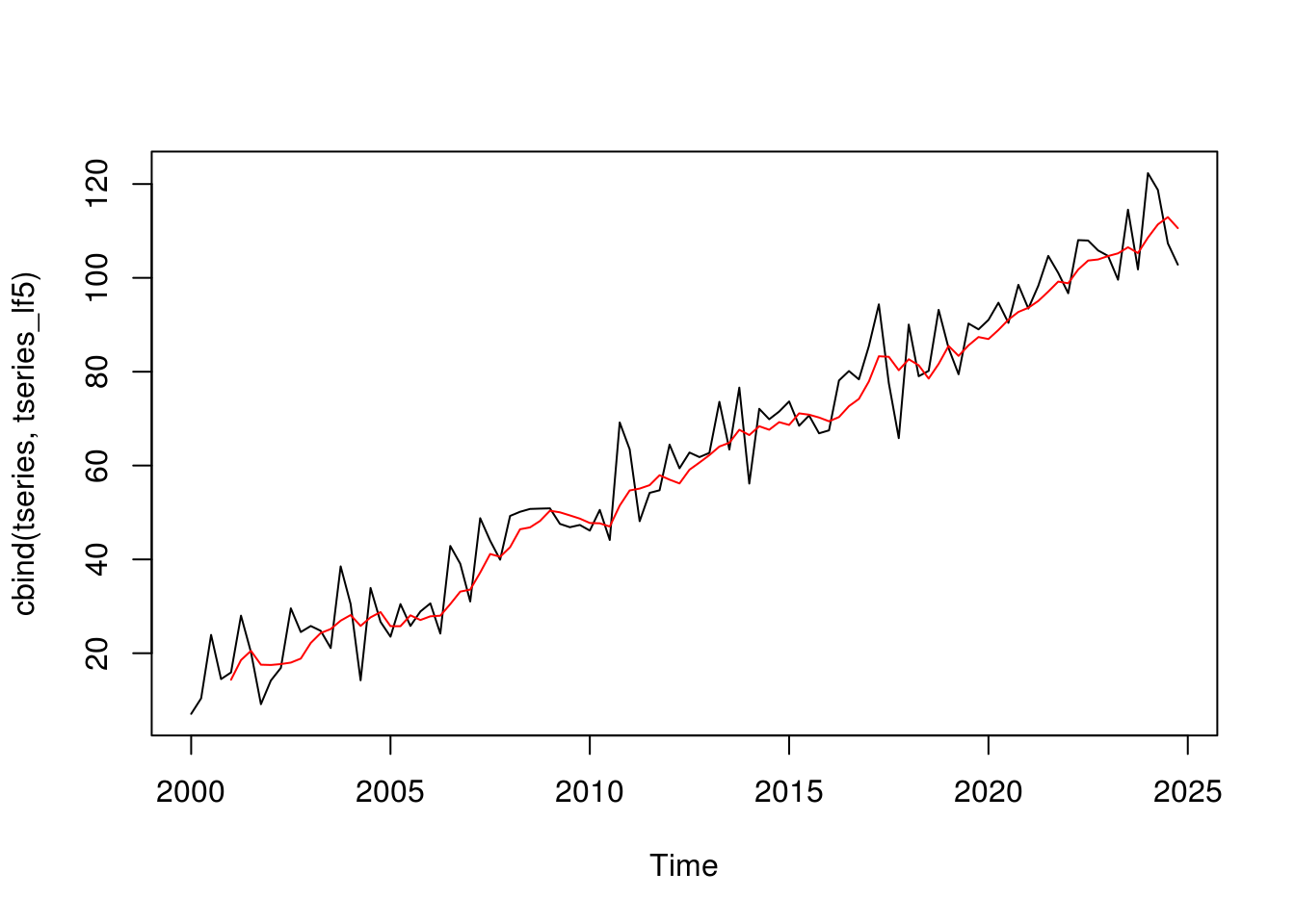
A moving average is another essential function for working with time series. For series with particularly high volatility, a moving average can help us to more clearly visualize its trend. Unfortunately, base R does not (to my knowledge) have a convenient function for calculating the moving average of a time series directly. However, we can use base R’s filter() function, which allows us to perform general linear filtering. We can set up the parameters of this function to be a moving average (Shumway and Stoffer, 2011). Here we apply the filter() function to tseries to create a 5 period moving average. The filter argument lets up specify the filter, which in this case is just a weighted average of 5 observations. The sides argument allows us to specify whether we want to apply the filter over past values (sides = 1), or to both past and future values (sides = 2). Here I set sides to 1 indicating that I want a trailing moving average:
tseries_lf5 <- filter(tseries, filter = rep(1/5, 5), sides = 1)
plot.ts(cbind(tseries, tseries_lf5), plot.type = 'single', col = c('black', 'red'))
The fact that we have to define the linear filter each time we use this function makes it a little cumbersome to use. If we don’t mind introducing a dependency to our code, we could use the SMA() function from the TTR package or the ma() function from the forecast package. The SMA() function takes a ts object and a value for n – the window over which we want to calculate the moving average.
library(TTR)
tseries_ma5 <- SMA(tseries, n = 5)
The ma() function from the forecast package also performs moving average calculations. We supply the time series and a value for the order argument.
tseries_ma5fore <- ma(tseries, order = 5)
Let’s compare the results. The SMA() function returns a trailing moving average where each value is the mean of the n most recent trailing values. This is equivalent to the results we get from using the filter() function. The ma() function from the forecast package returns a centered moving average. In this case tseries_ma5for is equal to the average of the current observation, the previous two observation, and the next two observations. Which one you use would depend on your application.
          tseries tseries_lf5 tseries_ma5 tseries_ma5fore
2000 Q1  7.076670          NA          NA              NA
2000 Q2 10.388758          NA          NA              NA
2000 Q3 23.910958          NA          NA        14.35499
2000 Q4 14.493559          NA          NA        18.54075
2001 Q1 15.905014    14.35499    14.35499        20.50828
2001 Q2 28.005455    18.54075    18.54075        17.55500
2001 Q3 20.226413    20.50828    20.50828        17.49470
2001 Q4  9.144571    17.55500    17.55500        17.68977
2002 Q1 14.192030    17.49470    17.49470        18.00239
2002 Q2 16.880366    17.68977    17.68977        18.86085
That’s it for Part 2. I don’t know about you, but I am sick of working with generated data. I want to work with some real world data. In Part 3 we’ll do just that using Quandl. See you then.
References
- Hyndman, Rob J. and George Athanasopoulos (2013) Forecasting: Principles and Practice. https://www.otexts.org/fpp
Shumway, Robert H. and David S. Stoffer (2011) Time Series Analysis and Its Applications With R Examples. New York, NY: Springer.
