Many datasets these days are collected at different locations over space which may generate spatial dependence. Spatial dependence (observation close together are more correlated than those further apart) violate the assumption of independence of the residuals in regression models and require the use of a special class of models to draw the valid inference.
The first thing to realize is that spatial data come in very different forms: areal data (murder rate per county), point pattern (trees in forest – random sampling locations) or point referenced data (soil carbon content – non random sampling locations), and all of these forms have specific models and R packages such as spatialreg for areal data or spatstat for point pattern.
In this blog post I will introduce how to perform, validate and interpret spatial regression models fitted in R on point referenced data using Maximum Likelihood with two different packages: (i) spaMM and (ii) glmmTMB. If you, reader, are aware of other packages out there to fit these models do let me know and I'll be happy to include it in this post.
Do I need a spatial model?
Before plugging into new model complexity, the first question to ask is: “do my dataset require me to take spatial dependence into account?”.
The basic steps to answer this question are:
- fit a non-spatial model (lm, glmer …)
- test for spatial autocorrelation in the residuals (Moran's I …)
3a. No indication of spatial dependence: fine to continue with your non-spatial model
3b. Indication of spatial dependence: fit a spatial model
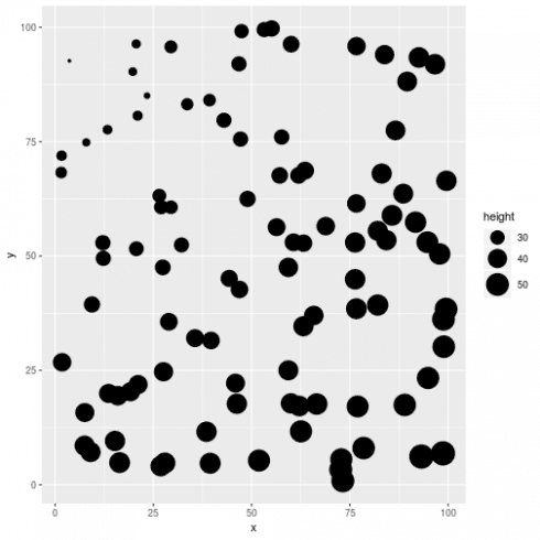
Let's look at this with a first simulated example. In a research project we are interested in understanding the link between tree height and temperature, to achieve this we recorded both parameters in 100 different forests and we want to use regression models.
Step 0: data simulation
# load libraries
library(tidyverse)
library(gridExtra)
library(NLMR)
library(DHARMa)

# simulate a random temperature gradient
temp <- nlm_distancegradient(ncol = 100, nrow = 100, origin = c(1,10,1,10), rescale = TRUE)

# extract the temperature values at 100 random points
dat <- data.frame(x = runif(100,0,100), y = runif(100,0,100))
dat$temperature <- raster::extract(temp, dat)

# simulate tree height
dat$height <- 20 + 35 * dat$temperature + rnorm(100)

# plot spatial pattern in tree height
ggplot(dat, aes(x = x, y = y, size = height)) +
  geom_point() +
  scale_size_continuous(range = c(1,10))
# clear spatial pattern
Step 1: fit a non-spatial model
# fit a non-spatial model
m_non <- lm(height ~ temperature, dat)
Step 2: test for spatial autocorrelation in the residuals
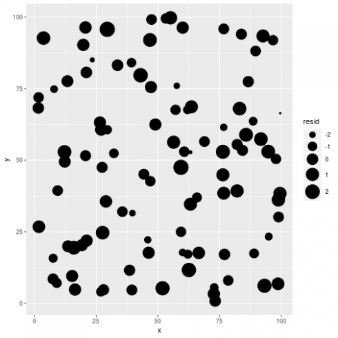
# plot residuals
dat$resid <- resid(m_non)
# dat$resid_std <- rescale(dat$resid, 1, 10)
ggplot(dat, aes(x = x, y = y, size = resid)) +
  geom_point() +
  scale_size_continuous(range = c(1,10))
Visually checking model residuals show that there seems to be little spatial dependency there. p-values fans can also rely on formal test (like Moran's I):
# formal test
sims <- simulateResiduals(m_non)
testSpatialAutocorrelation(sims, x = dat$x, y = dat$y, plot = FALSE)
##
##  DHARMa Moran's I test for spatial autocorrelation
##
## data:  sims
## observed = -0.020435, expected = -0.010101, sd = 0.016756, p-value
## = 0.5374
## alternative hypothesis: Spatial autocorrelation
No evidence of spatial Autocorrelation. We can go to Step 3a.
Step 3a
This little toy example showed that even if there are a spatial pattern in the data this does not mean that spatial regression models should be used. In some cases spatial patterns in the response variable are generated by spatial patterns present in the covariates, such as temperature gradient, elevation … Once we take into account the effect of these covariates spatial patterns in the response variable disappear.
So before starting to fit a spatial model, one should check that such complexity is warranted by the data.
Fitting a spatial regression model
The basic model structure that we will consider in this post is:
\[ y_i \sim \mathcal{N}(\mu_i, \sigma) \]
i index the different observations, y is the response variable (tree height …), \(\mu\) is the linear predictor and \(\sigma\) is the residual standard deviation. The linear predictor is defined as follow:
\[ \mu_i = X_i\beta + u(s_i) \]
The first term is just a classical regression in matrix notation (X is the design matrix and \(\beta\) is a vector of regression coefficient), the second term is the spatial term (correlated random term) defined as:
\[ u(s_i) \sim \mathcal{MVN}(0, F(\theta_1, …, \theta_n)) \]
The spatial term u(s) is basically a multivariate normal distribution with a mean vector of 0 and a covariance matrix given by some function with parameters to be estimated from the data. A classical choice is the Matérn function which has two parameters: \(\nu\) (control rate of decay, smaller value means faster decay) and \(\kappa\) (control smoothness, smaller values means lower smoothness). The input to the Matérn function are the distance between two points and the two parameters (\(\nu\) and \(\kappa\), as output we get the correlation matrix between the locations that will be used to get the spatial effect.
This model basically translate the expectation that closer observations should be more correlated, the strength of the spatial signal and its decay will have to be estimated from the data and we will explore here two packages to do so: spaMM and glmmTMB. I will show some code to fit the models, interpret the outputs, derive spatial predictions and check model assumptions for all three methods.
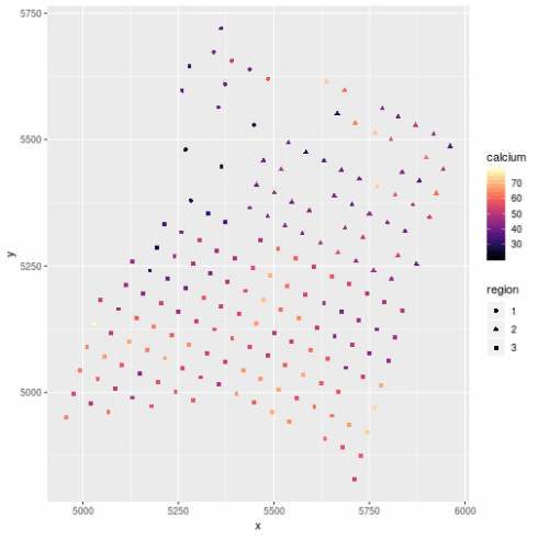
The dataset
library(geoR)
library(viridis)
data(ca20)
# put this in a data frame
dat <- data.frame(x = ca20$coords[,1], y = ca20$coords[,2], calcium = ca20$data, elevation = ca20$covariate[,1], region = factor(ca20$covariate[,2]))

# plot the data
ggplot(dat, aes(x=x, y = y, color =calcium, shape = region)) +
  geom_point() +
  scale_color_viridis(option = "A")
# fit a no-spatial model
m_lm <- lm(calcium ~ elevation + region, dat)
# test for spatial autocorrelation
sims <- simulateResiduals(m_lm)
testSpatialAutocorrelation(sims, dat$x, dat$y, plot = FALSE)
##
##  DHARMa Moran's I test for spatial autocorrelation
##
## data:  sims
## observed = 0.0594843, expected = -0.0056497, sd = 0.0069140,
## p-value < 2.2e-16
## alternative hypothesis: Spatial autocorrelation

# need to take into account space
spaMM
spaMM fits mixed-effect models and allow the inclusion of spatial effect in different forms (Matern, Interpolated Markov Random Fields, CAR / AR1) but also provide interesting other features such as non-gaussian random effects or autocorrelated random coefficient (ie group-specific spatial dependency). spaMM uses a syntax close to the one used in lme4, the main function to fit the model is fitme. We will fit the model structure outlined above to the calcium dataset:
library(spaMM)
# fit the model
m_spamm <- fitme(calcium ~ elevation + region + Matern(1 | x + y), data = dat, family = "gaussian") # this take a bit of time
# model summary
summary(m_spamm)
## formula: calcium ~ elevation + region + Matern(1 | x + y)
## ML: Estimation of corrPars, lambda and phi by ML.
##     Estimation of fixed effects by ML.
## Estimation of lambda and phi by 'outer' ML, maximizing p_v.
## Family: gaussian ( link = identity )
##  ------------ Fixed effects (beta) ------------
##             Estimate Cond. SE t-value
## (Intercept)  34.6296   10.311  3.3585
## elevation     0.8431    1.860  0.4534
## region2       8.1300    5.062  1.6060
## region3      14.5586    4.944  2.9448
##  --------------- Random effects ---------------
## Family: gaussian ( link = identity )
##                    --- Correlation parameters:
##       1.nu      1.rho
## 0.43286763 0.01161491
##            --- Variance parameters ('lambda'):
## lambda = var(u) for u ~ Gaussian;
##    x + y  :  105.3
## # of obs: 178; # of groups: x + y, 178
##  ------------- Residual variance  -------------
## phi estimate was 0.0030988
##  ------------- Likelihood values  -------------
##                         logLik
## p_v(h) (marginal L): -628.6316
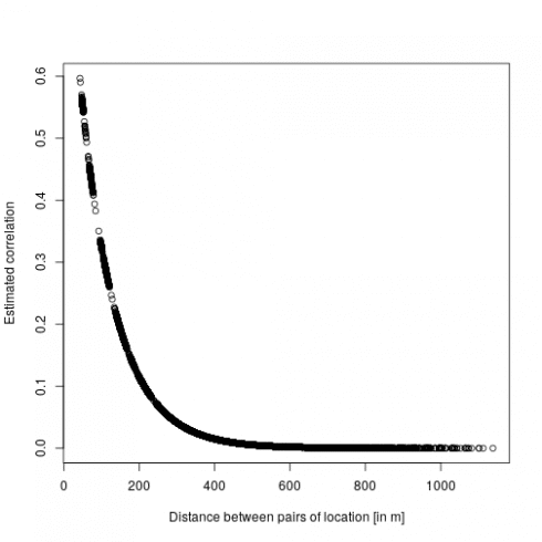
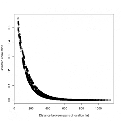
There are two main output interesting here: first are the fixed effect (beta) which are the estimated regression parameters (slopes). Then the correlation parameter nu and rho which represent the strength and the speed of decay in the spatial effect, which we can turn into the actual spatial correlation effect by plotting the estimated correlation between two locations against their distance:
dd <- dist(dat[,c("x","y")])
mm <- MaternCorr(dd, nu = 0.43, rho = 0.01)
plot(as.numeric(dd), as.numeric(mm), xlab = "Distance between pairs of location [in m]", ylab = "Estimated correlation")
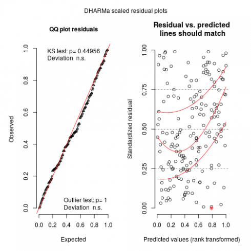
So basically locations more than 200m away have a correlation below 0.1. Now we can check the model using DHARMa:
sims <- simulateResiduals(m_spamm)<
## Warning in checkModel(fittedModel): DHARMa: fittedModel not in class of
## supported models. Absolutely no guarantee that this will work!
## Unconditional simulation:
plot(sims)
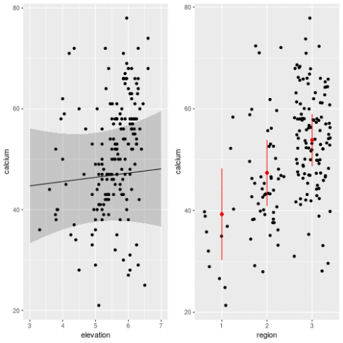
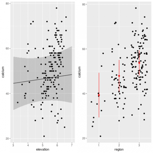
Looks relatively ok. Now we can predict the effect of elevation and region while controlling for spatial effects:
# the effect of elevation
newdat <- expand.grid(x = 5000, y = 5200, elevation = seq(3, 7, length.out = 10), region = factor(1, levels = c(1:3)))

newdat$calcium <- as.numeric(predict(m_spamm, newdat, re.form = NA)) # re.form = NA used to remove spatial effects
newdat$calcium <- newdat$calcium + mean(c(0,fixef(m_spamm)[3:4])) # to remove region effect
# get 95% confidence intervals around predictions
newdat <- cbind(newdat, get_intervals(m_spamm, newdata = newdat, intervals = "fixefVar", re.form = NA) + mean(c(0,fixef(m_spamm)[3:4])))


gg1 <- ggplot(dat, aes(x = elevation, y = calcium)) +
  geom_point() +
  geom_path(data = newdat) +
  geom_ribbon(data = newdat, aes(ymin = fixefVar_0.025, ymax = fixefVar_0.975), alpha = 0.2)

# now for region effect
newdat <- data.frame(x = 5000, y = 5200, elevation = mean(dat$elevation), region = factor(1:3)) # averaging out elevation effect
newdat$calcium <- as.numeric(predict(m_spamm, newdat, re.form = NA))
# get 95% CI
newdat <- cbind(newdat,get_intervals(m_spamm, newdata = newdat, intervals = "fixefVar", re.form = NA))

gg2 <- ggplot(dat, aes(x = region, y = calcium)) +
  geom_jitter() +
  geom_point(data = newdat, color = "red", size = 2) +
  geom_linerange(data = newdat, aes(ymin = fixefVar_0.025, ymax = fixefVar_0.975), color = "red")

# plot together
grid.arrange(gg1, gg2, ncol = 2)
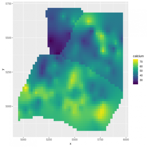
We can also derive prediction at any spatial location provided that we feed in information on the elevation and the region:
library(fields)
library(raster)
# derive a DEM
elev_m <- Tps(dat[,c("x","y")], dat$elevation)
## Warning:
## Grid searches over lambda (nugget and sill variances) with  minima at the endpoints:
##   (GCV) Generalized Cross-Validation
##    minimum at  right endpoint  lambda  =  5.669116e-06 (eff. df= 169.1 )
r <- raster(xmn = 4950, xmx = 5970, ymn = 4800, ymx = 5720, resolution = 10)
elev <- interpolate(r, elev_m)

# for the region info use the limits given in ca20
pp <- SpatialPolygons(list(Polygons(list(Polygon(ca20$reg1)), ID = "reg1"),Polygons(list(Polygon(ca20$reg2)), ID = "reg2"), Polygons(list(Polygon(ca20$reg3)), ID = "reg3")))
region <- rasterize(pp, r)

# predict at any location
newdat <- expand.grid(x = seq(4960, 5960, length.out = 50), y = seq(4830, 5710, length.out = 50))
newdat$elevation <- extract(elev, newdat[,1:2])
newdat$region <- factor(extract(region, newdat[,1:2]))
# remove NAs
newdat <- na.omit(newdat)
# predict
newdat$calcium <- as.numeric(predict(m_spamm, newdat))

(gg_spamm <- ggplot(newdat,aes(x=x, y=y, fill = calcium)) +
  geom_raster() +
  scale_fill_viridis())
That's it for spaMM a great, fast and easy way to fit spatial regressions.
glmmTMB
glmmTMB fits a broad class of GLMM using Template Model Builder. With this package we can fit different covariance structure including spatial Matern. Let's dive right in.
library(glmmTMB)
# fitst we need to create a numeric factor recording the coordinates of the sampled locations
dat$pos <- numFactor(scale(dat$x), scale(dat$y))
# then create a dummy group factor to be used as a random term
dat$ID <- factor(rep(1, nrow(dat)))

# fit the model
m_tmb <- glmmTMB(calcium ~ elevation + region + mat(pos + 0 | ID), dat) # take some time to fit
# model summary of fixed effects
summary(m_tmb)
##  Family: gaussian  ( identity )
## Formula:          calcium ~ elevation + region + mat(pos + 0 | ID)
## Data: dat
##
##      AIC      BIC   logLik deviance df.resid
##   1272.9   1298.4   -628.5   1256.9      170
##
## Random effects:
##
## Conditional model:
##  Groups   Name                                        Variance  Std.Dev.
##  Corr
##
##  [ reached getOption("max.print") -- omitted 179 rows ]
## Number of obs: 178, groups:  ID, 1
##
## Dispersion estimate for gaussian family (sigma^2): 0.0277
##
## Conditional model:
##             Estimate Std. Error z value Pr(>|z|)
## (Intercept)  33.9307    10.4800   3.238  0.00121 **
## elevation     0.9764     1.9097   0.511  0.60917
## region2       8.5945     5.2265   1.644  0.10010
## region3      14.4099     5.4326   2.652  0.00799 **
## ---
## Signif. codes:  0 '***' 0.001 '**' 0.01 '*' 0.05 '.' 0.1 ' ' 1
The output from glmmTMB should be familiar to frequent users of lme4, first we have some general model information (family, link, formula, AIC …), then we have the estimation of the random effect variance (estimated at 105 here very close to the value from spaMM), and the last table under “Conditional model” display the estimates for the fixed effects. These are again pretty close to those estimated by spaMM.
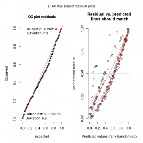
Before going any further let's check the model fitness.
sims <- simulateResiduals(m_tmb)
plot(sims)
By running these lines we get a warning that glmmTMB does not implement yet unconditional predictions (without random effect) is not yet possible in glmmTMB so one may expect (and we do see) some upward going slopes on the right graphs. Not much to do at this stage, maybe in the (near) future with update to glmmTMB this could be solved.
We can look at the predicted spatial effect:
# some R magic to extract and re-order the estimated correlation between pairs of locations
fit_cor <- matrix(as.numeric(attr(VarCorr(m_tmb)$cond$ID, "correlation")), nrow = 178, ncol = 178, byrow = FALSE,
                  dimnames = attr(attr(VarCorr(m_tmb)$cond$ID, "correlation"),"dimnames"))

ff <- dimnames(fit_cor)[[1]]
ff <- gsub("pos","",ff)
fit_cor2 <- fit_cor[order(match(ff, dat$pos)), order(match(ff, dat$pos))]

# plot
plot(as.numeric(dd), fit_cor2[lower.tri(fit_cor2)],
     xlab = "Distance between pairs of location [m]",
     ylab = "Estimated correlation")
We find here a similar picture to the one from spaMM, but this was quite a bit more work to get it and we don't seem to have direct estimation of the Matern parameters that were readily available in spaMM. We can now look at the effect of elevation and region (since there is no way to marginalize over the random effects in glmmTMB we have to get the CI by hand):
# the effect of elevation
newdat <- data.frame(elevation = seq(3, 7, length = 10), region = factor(1, levels = 1:3))
# turn this into a model matrix
mm <- model.matrix(~ elevation + region, newdat)
newdat$calcium <- mm %*% fixef(m_tmb)$cond + mean(c(0, fixef(m_tmb)$cond[3:4])) # predicted values removing region effects
pvar <- diag(mm %*% tcrossprod(vcov(m_tmb)$cond, mm))
newdat$lci <- newdat$calcium - 1.96 * sqrt(pvar)
newdat$uci <- newdat$calcium + 1.96 * sqrt(pvar)

gg1 <- ggplot(dat, aes(x = elevation, y = calcium)) +
  geom_point() +
  geom_line(data = newdat) +
  geom_ribbon(data = newdat, aes(ymin = lci, ymax = uci), alpha = 0.2)

# the effect of region
newdat <- data.frame(elevation = mean(dat$elevation), region = factor(1:3))
# turn this into a model matrix
mm <- model.matrix(~ elevation + region, newdat)
newdat$calcium <- mm %*% fixef(m_tmb)$cond # predicted values
pvar <- diag(mm %*% tcrossprod(vcov(m_tmb)$cond, mm))
newdat$lci <- newdat$calcium - 1.96 * sqrt(pvar)
newdat$uci <- newdat$calcium + 1.96 * sqrt(pvar)

gg2 <- ggplot(dat, aes(x = region, y = calcium)) +
  geom_jitter() +
  geom_point(data = newdat, color = "red", size = 2) +
  geom_linerange(data = newdat, aes(ymin = lci, ymax = uci), color = "red")

# plot together
grid.arrange(gg1, gg2, ncol = 2)
Looks very close to the picture we got from spaMM, which is reassuring. It is a bit more laborious to get estimation of Confidence Intervals for glmmTMB as of know but in th enear future new implementation of the predict method with a “re.form=NA” argument would allow easier derivation of the CIs. Now let's see how to derive spatial predictions:
# predict at any location
newdat <- expand.grid(x = seq(4960, 5960, length.out = 50), y = seq(4830, 5710, length.out = 50))
newdat$ID <- factor(rep(1, nrow(newdat)))
newdat$elevation <- extract(elev, newdat[,1:2])
newdat$region <- factor(extract(region, newdat[,1:2]))
# remove NAs
newdat <- na.omit(newdat)
newdat$pos <- numFactor(((newdat$x - mean(dat$x)) / sd(dat$x)), ((newdat$y - mean(dat$y)) / sd(dat$y)))
# predict in slices of 100 predictions to speed up computation
pp <- rep(NA, 1927)
for(i in seq(1, 1927, by = 100)){
  if(i == 1901){
    pp[1901:1927] <- predict(m_tmb, newdat[1901:1927,], allow.new.levels = TRUE)
  }
  else{
    pp[i:(i+99)] <- predict(m_tmb, newdat[i:(i+99),], allow.new.levels = TRUE)
  }
  # print(i)
}
newdat$calcium <- pp
(gg_tmb <- ggplot(newdat,aes(x=x, y=y, fill = calcium)) +
  geom_raster() +
  scale_fill_viridis())
Very similar map to spaMM.
Conclusion
Time to wrap up what we've seen here. First off, before plunging into spatial regression models you should first check that your covariates do not already take into account the spatial patterns present in your data. Remember that in the implementation of the spatial models discussed here, spatial effects are modelled in a similar fashion to random effects (basically random effect take into account structure in the data be it by design or spatial or temporal structure). So any variation (including spatial) that can be explained by the fixed effects will be taken into account and only remaining variation based on the spatial structure will be effectively going into the estimated spatial effects.
Now I presented here two ways to fit similar spatial regression models in R, time to compare a bit their performance and their pros and cons.
- spaMM is a very nice package, it can handle a relatively large range of response distributions and can fit different form of spatial effects, it implements a synthax close to the classical lme4 one, and in the example tested here it fitted the model relatively fast. It also provides methods to derive predictions and confidence intervals and the general-purpose model checking package DHARMa works with spaMM objects.
- glmmTMB is a multi-purpose GLMM fitting package with a few extension into structured covariance matrices including spatial effects. The biggest issues with glmmTMB for spatial data are that model fitting is particularly slower than spaMM, deriving unconditional predictions (without spatial effects) is currently not possible and so DHARMa does not work properly and we need to do some stats wizardy to interprete and predict from a fitted model.
In a second part we will explore Bayesian ways to do spatial regression in R with the same dataset, stay tuned for more fun!
