Introduction
In this second part we will present a numerical method for solving the PDE system, which describes the propagation of action potential. We will make use of the R-Packages deSolve and ReacTran to simulate the model. The underlying Hodgkin-Huxley model used for our simulation is actually based on the telegraph equations. In contrast to the standard models, where the inductance is nelegted, here we will also use the Hodgkin-Huxley model but without neglecting the self conductance of the axon Isn’t there an inductance factor in the plasma membrane of nerves?. This model is based on the \((RLC)\)(Resistance-Inductance-Capacitance) electric circuit analogue in which ionic currents through the cylindrical membrane are also taken into account.
Propagation Action Potential
The mathematical equation describing the propagation in space and time of the action potential \(V_m\) along a neural axon is given by :
$$ \begin{align}\frac{\partial^2 V_m}{\partial^2x}- LC_a\frac{\partial^2V_m}{\partial^2t}= \frac{2}{a}RC_a\frac{\partial V_m}{\partial t} + \frac{2}{a}L\frac{\partial I_{}ion}{\partial t} + \frac{2}{a}RI_{ion} \hspace{30pt} (C.6)\end{align} $$
Where:
\(V_m\) is the potential difference across the membrane (dependent variable, depends on \(x\) and \(t\)).
\(x \) is independent variable representing one dimension of three-dimensional space.
\(t\) is independent variable representing time.
\(L\) is the axon specific self-inductance.
\(R\) is the specific resistance of an axon.
\(C_a\) is the axon self-capacitance per unit area per unit length.
\(I_{ion}\) is the sum of ions currents.
\(a\) is the axon radius.
The derivation of the equation \((C.6)\) for axon represented by the \(RLC\) (Resistance-Inductance-Capacitance) circuit is performed in Appendix A (In case you are interested in the derivation of the equation \((C.6)\) so just send me a mail at kritiker2017@gmail.com.). Note if the presence of induction in the system is neglected \((L=0)\), the equation \((C.6)\) becomes the non-linear cable equation, which is not resistant to analytical approaches.
In the Hodgkin-Huxley model the ion current \(I_{ion}\) is defined as the sum of ions currents of potassium and sodium ( \(I_K\) and \(I_{Na}\)), and a smaller current (\(I_L\) ) made up of chloride and other ions:
$$I_{ion} = I_K + I_{Na} + I_L= g_K(V_m -V_K)+g_{Na}(V_m – V_{Na}) + g_L(V_m – V_L) \hspace{30pt} (C.7)$$ where \(g_K\) , \(g_{Na}\) and \(g_L\) are potassium, sodium and leakage conductances, respectively.
We define:
the diffusion coefficient as \(D^2 = \frac{a}{2LC_m}\)
the relaxation time as \(\tau = \frac{L}{R}\)
the parameter \(\mu = \frac{\tau}{C_m}\) characterizes the inductance in the system.
Substituting the equation \((C.7)\) into equation \((C.6)\) we obtain the final nerve propagation equation in the Hodgkin & Huxley model, which will be used for our simulation.
$$
\begin{align}\tau\frac{\partial^2 V_m}{\partial^2t} = \tau D^2\frac{\partial^2 V_m }{\partial^2 x} – \big[1+\mu(g_{K}n^4 + g_{Na}m^3h+g_{L})\big]\frac{\partial V_m}{\partial t} – \\ g_{K}(\frac{\mu}{\tau}n^4 + 4\mu n^3\frac{\partial n}{\partial t})(V_m – V_K)
– \\ g_{Na}\big[\frac{\mu}{\tau}m^3h + \mu(3m^2h\frac{\partial m}{\partial t}+ m^3\frac{\partial h}{\partial t}) \big](V_m – V_{Na}) – \\ g_L\frac{\mu}{\tau}(V_m – V_L) \hspace{40pt} (C.8)\end{align} $$
Numeric solution
To solve the equation \((C.8)\) we will make use of the R-Packages {deSolve} and {ReacTran}. The [Package deSolve is an add-on package of the open source data analysis system R for the numerical treatment of systems of differential equations.].
In this blog post we solve the equation \((C.8)\) on a one-dimensional domain \(\Omega = [0,15]\), with the initial conditions \(V_{m}(x, 0) = -15 \exp{-\frac{x^2}{D^2}}\) and \(\frac{\partial V_{m}(x,0)}{\partial t} = 0 \) and boundary conditions of Dirichlet type \( V_{m}(x = 0, t) = 0\), \(V_{m}(x = 15, t) = 0\). The “method of lines”, where space(\(\Omega\)) is discretized in fixed steps while time is left in continuous form, will be used.
library(ReacTran)
  # Create one-dimensional finite difference grid
  dx <- 1
  xgrid <- setup.grid.1D(x.up = 0, x.down = 10, dx.1 = dx)
  x <- xgrid$x.mid
  N <- xgrid$N
  # Model Parameters
  ## Passive parameters of the neuron
  a <- 238*10^(-4) # axon radius (cm)
  R <- 35.4        # Membrane Capacitance (Ohm cm)
  L <- 15          # Axon specific self-inductance
  C_m <- 0.001     # Membrane capacitance density Cm 1.0 micro F/cm2
  D_coefficient <- sqrt(a/(2*L*C_m))
  tau <- L/R
  mu <- tau/C_m
  Iinj <- 0       # injected current
  # Values of the neuron
  g_K  <- 0.036       # conductance density g_K
  g_Na <- 0.12        # conductance density g_Na
  g_L  <- 0.0003      # conductance density g_L
  v_K  <- 12          # K reversal potential
  v_Na <- -115        # Na reversal potential
  v_L <- -10.5989     # Leak reversal potential
  # Function ion Channel
  ## Rate functions for K activation (variable n)
  alpha_n <- function(v) 0.01*(v+10)/(-1+exp((v+10)/10))
  beta_n  <- function(v) 0.125*exp(v/80)
  ## Rate functions for Na activation (variable m)
  alpha_m <- function(v) 0.1*(v+25)/(-1+exp((v+25)/10))
  beta_m  <- function(v) 4*exp(v/18)
  # Rate functions for Na inactivation (variable h)
  alpha_h <- function(v) 0.07*exp(v/20)
  beta_h  <- function(v) (1+exp((v+30)/10))^-1
  # Derivatives of ion channel functions/Kinetic equations for channel variables
  dndt <- function(n,v)(alpha_n(v)*(1-n)-beta_n(v)*n)
  dmdt <- function(m,v)(alpha_m(v)*(1-m)-beta_m(v)*m)
  dhdt <- function(h,v)(alpha_h(v)*(1-h)-beta_h(v)*h)
  # Initial conditions
  ## In the resting state V = 0
  V_0  <- 0
  n_0  <- alpha_n(V_0)/(alpha_n(V_0)+beta_n(V_0))
  m_0  <- alpha_m(V_0)/(alpha_m(V_0)+ beta_m(V_0))
  h_0  <- alpha_h(V_0)/(alpha_h(V_0)+beta_h(V_0))
  vini <- (-15)*exp(-x^2/D_coefficient^2)
  # vini <- -15*sin(pi*x)
  # vini <- rep(-15, N)
  uini  <- rep(0, N)
  nini  <- rep(n_0, N)
  mini  <- rep(m_0, N)
  hini  <- rep(h_0, N)
  yini  <- c(vini, uini, nini, mini, hini)
  # Model equations/Differential equations
  Pulse_propagation <- function (t, y, parms) {
    v <- y[1:N]
    u <- y[(N+1):(2*N)]
    n <- y[(2*N+1):(3*N)]
    m <- y[(3*N+1):(4*N)]
    h <- y[(4*N+1):(5*N)]

    dv <- u
    du <- tran.1D(C = v, C.up = 0, C.down = 0,  D = D_coefficient, dx = xgrid)$dC -
      (1/tau + (mu/tau)*(g_K*n^4 + g_Na*m^3*h + g_L))*u -
      g_K*((mu/tau^2)*n^4 + 4*(mu/tau)*n^3*dndt(n,v))*(v-v_K) -
      g_Na*((mu/tau^2)*m^3*h + (mu/tau)*(3*m^2*h*dmdt(m,v) + m^3*dhdt(h,v)))*(v -v_Na) -
      g_L*(mu/tau^2)*(v - v_L) + Iinj

    dn <- (alpha_n(v)*(1-n)-beta_n(v)*n)
    dm <- (alpha_m(v)*(1-m)-beta_m(v)*m)
    dh <- (alpha_h(v)*(1-h)-beta_h(v)*h)
    return(list(c(dv,du, dn, dm, dh)))
  }
We’ve done with building the model. In the above model code the action potential \(V_m\) is represented by the state variable v, which represents the dynamical attitude of the transmission for the nerve impulses of a nervous system. We define now the time simulation and run the model to solve the equation \((C.8)\).
 # Specify the time at which the output is wanted
  time_3 <- seq(0,15, 0.01)
The defined model is one-dimensional (one spatial independent variable), so we use the function ode.1D here. The time it takes to solve the model (in seconds) is also printed.
 print(system.time(
    out_3 <- ode.1D(y = yini, func = Pulse_propagation,
                    times = time_3, method = "adams", parms = NULL,
                    dimens = N, nspec = 5,
                    names = c("v", "u", "n", "m", "h"))))
       User      System     verstrichen
       0.21        0.00        0.20
The model output/results “out_3” is a matrix, which contains all the data needed to analyse and visualize the results of the simulation.
Before plotting the numeric solution of the PDE \((C.8)\), we will first check if the integration was successful, and to get detailed information about the success of our simulation we use the function diagnostics{deSolve} and the function summary{deSolve}
Diagnostics and Summary
# Print detailed information about the success of our
  diagnostics(out_3)
--------------------
lsode return code
--------------------

  return code (idid) =  2
  Integration was successful.

--------------------
INTEGER values
--------------------

  1 The return code : 2
  2 The number of steps taken for the problem so far: 1950
  3 The number of function evaluations for the problem so far: 2120
  5 The method order last used (successfully): 4
  6 The order of the method to be attempted on the next step: 4
  7 If return flag =-4,-5: the largest component in error vector 0
  8 The length of the real work array actually required: 820
  9 The length of the integer work array actually required: 20
 14 The number of Jacobian evaluations and LU decompositions so far: 0

--------------------
RSTATE values
--------------------

  1 The step size in t last used (successfully): 0.01
  2 The step size to be attempted on the next step: 0.01
  3 The current value of the independent variable which the solver has reached: 15.00627
  4 Tolerance scale factor > 1.0 computed when requesting too much accuracy: 0
  summary(out_3)

                    v             u            n            m            h
Min.    -1.052214e+02 -3.101267e+02 3.176769e-01 1.396179e-02 7.750275e-02
1st Qu. -2.231145e+00 -1.013699e+00 3.177112e-01 2.289523e-02 2.584720e-01
Median  -4.608204e-06 -7.997909e-02 3.706068e-01 5.293269e-02 5.108495e-01
Mean    -8.208256e+00  5.239505e-01 4.551956e-01 1.883197e-01 4.269989e-01
3rd Qu.  7.670459e+00  4.150809e-06 5.910743e-01 7.744576e-02 5.960693e-01
Max.     1.204040e+01  7.670492e+01 7.681718e-01 9.940305e-01 5.961208e-01
N        1.501000e+04  1.501000e+04 1.501000e+04 1.501000e+04 1.501000e+04
sd       2.720432e+01  3.933037e+01 1.595711e-01 3.139004e-01 1.858227e-01
Plot the results
Time evolution of membrane potential of H&H neuron at various distances along the axon.
As we can see in the following plot, when an excitable membrane is incorporated into a nonlinear equation \((C.6)\) and we use accommodated initial and boundary conditions, the model can give rise to traveling waves of electrical excitation and the action potential repeats itself at successive locations along the axon. The magnitude and duration of action potential remains the same throughout the propagation along the neuron’s axon.
 library(plotly)
  library(see)
  # Gather columns into key-value pairs
  ldata % tidyr::gather(Shape, Action_Potential, -time)
  # head(ldata)
  ldata_1_9 %filter(Shape == (1):(N-1))
  plot_ldata <- ggplot(ldata_1_9,
         aes(x = time,
             y = - Action_Potential,
             group = Shape,
             col = Shape
             )) + labs(title = "Action Potential profiles through time \n at various axon distances") + geom_line() + theme_abyss() # + geom_hline(yintercept = 15, color = "red", lwl =2)
  ggplotly(plot_ldata)
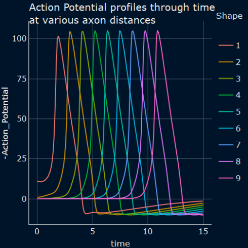
Figure 1: Numerical solution of equation \((C.8)\) showing the time course of action potential. The action potential repeats itself at successive locations along the axon.
3D Plot of the numeric solution
To visualize the results in 3D the R version of the package{plotly} is used.
 action_potential <- subset(out_3, which = c("v"))
  fig_surface %
    layout(title = list(text = " 3D Plot of the numeric solution", y = 0.95 ), scene = list(
            xaxis = list(title = "Distance"),
            yaxis = list(title = "Time"),
            zaxis = list(title = "v: Action Potential")
            )
           )
  fig_surface
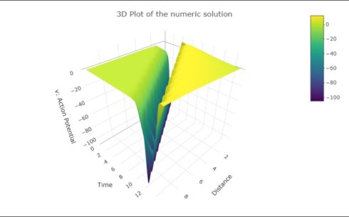
Figure 2: 3D Presentation of the numerical solution of equation \((C.8)\).
The following plots are showing the time course of the other dependent variables, n, m, h and dv/dt.
Plot_all_gatting <- function(x,y, my_title){
    library(plotly)
    library(see)
      ldata %tidyr::gather(Shape, variable, -time)
    # head(ldata)
      ldata_1_9 %filter(Shape == x:y)
      plot_ldata <- ggplot(ldata_1_9, aes(x = time, y = variable , group = Shape, col = Shape )) +
      labs(title = my_title ) +
       geom_line() + theme_radar_dark()
      }
  n <- Plot_all_gatting(2*N+1, 3*N, "n profiles through time \n at various axon distances")
  m <- Plot_all_gatting(3*N+1,4*N, "m profiles through time \n at various axon distances")
  h <- Plot_all_gatting(4*N+1,5*N, " h profiles through time \n at various axon distances")
  u <- Plot_all_gatting(N+1, 2*N, "dV/dt profiles through time \n at various axon distances")
  gridExtra::grid.arrange(n, m, h, u, ncol =2)
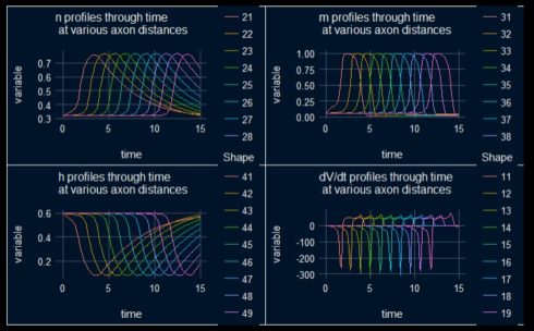
Figure 3: Time courses of dv/dt and the gating functions n,m,h.
3D Plots of action Potential, and the gating variables n,m,h
dVdt <- subset(out_3, which = c("u"))
  M <-   subset(out_3, which = c("m"))
  N <-   subset(out_3, which = c("n"))
  H <-   subset(out_3, which = c("h"))
  # custom grid style
  axx <- list(
    gridcolor='rgb(255, 255, 255)',
    zerolinecolor='rgb(255, 255, 255)',
    showbackground= TRUE,
    backgroundcolor='rgb(230, 230,230)')

  # individual plots
  fig1 <- plot_ly(x = x, y = time_3,  z = - dVdt , scene='scene')
  fig1 % add_surface(showscale=FALSE)

  fig2 <- plot_ly(x = x, y = time_3,z = M, scene='scene2')
  fig2 % add_surface(showscale=FALSE)

  fig3 <- plot_ly(x = x, y = time_3,z = N, scene='scene3')
  fig3 % add_surface(showscale=FALSE)

  fig4 <- plot_ly(x = x, y = time_3,z = H, scene='scene4')
  fig4 % add_surface(showscale=FALSE)

  # subplot and define scene
  fig <- subplot(fig1, fig2, fig3, fig4)
  fig % layout(title = "3D Plots of the numeric solution for dv/dt, n,m and h",
                        scene = list(domain=list(x=c(0,0.5),y=c(0.5,1)),
                                     xaxis = c(axx, list(title = "Distance")),
                                     yaxis = c(axx, list(title = "Time")),
                                     zaxis = c(axx, list(title = "dv/dt")),
                                     aspectmode='cube'),
                        scene2 = list(domain=list(x=c(0.5,1),y=c(0.5,1)),
                                      xaxis = c(axx, list(title = "Distance")),
                                      yaxis = c(axx, list(title = "Time")),
                                      zaxis = c(axx, list(title = "Gatting \n variable m")),
                                      aspectmode='cube'),
                        scene3 = list(domain=list(x=c(0,0.5),y=c(0,0.5)),
                                      xaxis = c(axx, list(title = "Distance")),
                                      yaxis = c(axx, list(title = "Time")),
                                      zaxis = c(axx, list(title = "Gatting \n variable n")),
                                      aspectmode='cube'),
                        scene4 = list(domain=list(x=c(0.5,1),y=c(0,0.5)),
                                      xaxis = c(axx, list(title = "Distance")),
                                      yaxis = c(axx, list(title = "Time")),
                                      zaxis = c(axx, list(title = "Gatting \n variable h")),
                                      aspectmode='cube'))


  fig
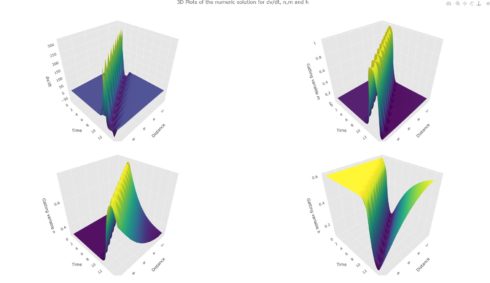
Fig 4: 3D representation of the numerical solution of dv/dt, n, m and h.
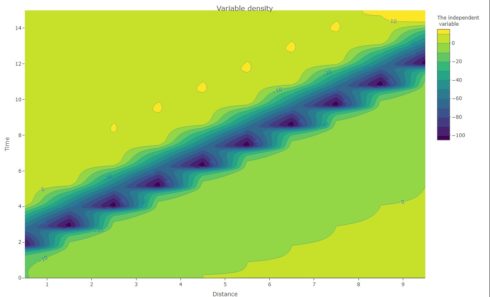
and finally the contour plot
Contour Plot
 action_potential <- subset(out_3, which = "v")
  fig_prop <- plot_ly(visible = TRUE,
                 x = x ,
                 y = time_3,
                 z = action_potential,
                 type = "contour", contours = list(showlabels = TRUE))
  fig_prop % colorbar(title = "The independent \n variable") %>%
    layout(title = list(text = "Variable density", y = 0.98), xaxis = list(title = "Distance "), yaxis = list(title =  "Time" ))
  fig_prop
Shiny application
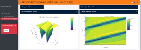
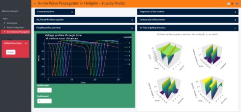
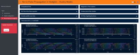
Using my new Shiny application (not yet published, it is still under development), one can explore the spatiotemporal dynamics of the action potential and the ionic currents. Just to show an example, when we change the initial value of the action potential in the Shiny application to -65mv (instead of -15mv in the above model) the model produces more than one spike and generates a periodic response. With this app one can also study the influence of the axon specific self-inductance on the spatiotemporal dynamics of the action potential and its proprieties (all-or-none rule, ….). In the Shiny application if we change the initial value of the action potential and then just click the update button, so one can get the results as shown below:
Summary and Outlook
In this blog post we solved the one dimensional PDE using only R-Packages, this hyperbolic PDE is describing the dynamics of the action potential along an axon. Our numerical solution shows the well known results, namely the transmission/production of the action potential along the axon does not change its magnitude and shape.
Next I will investigate a more realistic model, the two dimension nerve pulse propagation model.
References
- Mathematical Modelling of Nerve Pulse Transmission : https://core.ac.uk/download/pdf/236625972.pdf
- Cable Theory: https://pages.jh.edu/motn/coursenotes/cable.pdf
- Solving Differential Equations in R :
https://www.researchgate.net/publication/41530790_Solving_Differential_Equations_in_R_Package_deSolve - Plotly in R: https://plotly.com/r/getting-started
- Creating Shiny Application with bs4Dash: https://rinterface.github.io/bs4Dash/index.html
Contact:
kritiker2017@gmail.com.
