Please read the first part published at DS+, if you haven’t. Effect sizes and the strength of our prediction: One relatively common question in statistics or data science is, how “big” is the difference or the effect? At this point, we can state with some statistical confidence that tire brand matters in predicting tire mileage life, it isn’t likely given our data that we would see results like these by chance.
But… Is this a really big difference between the brands? Often this is the most important question in our research. After all, if it’s a big difference we might change our shopping habits and/or pay more. Is there a way of knowing how big this difference is?
Effect size is a measure we use in statistics to express how big the differences are. For this Oneway ANOVA the appropriate measure of effect size is eta squared (\(\eta^2\)) which can be calculated as:
\[\eta^2 = \frac{SS_{between}}{SS_{total}}\]
So while our F value is the ratio of brand and residuals of the mean squares, \(\eta^2\) is between over total for the sums of squares. Essentially, \(\eta^2\) is a measure of how much of the total variation in our data we can attribute to Brand and how much is just good old-fashioned random variation. If \(\eta^2\) is one (which would be suspicious with real data) then 100% of the data is explainable if you know the brand. The more variance you explain the bigger the effect.
So how to get the number \(\eta^2\) from our data? We could just go back and do the work manually, you can see an example of that in LSR in section 14.2.5. You can save a LOT of typing by using this equivalent formula \(\eta^2\) = var(predict(tyres.aov)) / var(tyre$Mileage) = 0.4900957 . But that looks tedious to type even once so let’s use the etaSquared function provided in lsr.
ETASQUARED <- var(predict(tyres.aov)) / var(tyre$Mileage)
ETASQUARED
## [1] 0.4900957
etaSquared(tyres.aov)
##           eta.sq eta.sq.part
## Brands 0.4900957   0.4900957
round(etaSquared(tyres.aov,anova = TRUE),2) # tidy up a bit include full table
##           eta.sq eta.sq.part     SS df    MS     F  p
## Brands      0.49        0.49 256.29  3 85.43 17.94  0
## Residuals   0.51          NA 266.65 56  4.76    NA NA
So our value for eta squared is \(\eta^2\) = 0.4900957 . Obviously you should exercise professional judgment in interpreting effect size but it does appear that brand matters… Eta squared is even more useful as we add more factors to our ANOVA and allows us to make direct comparisons about factors relative contributions to explanation.
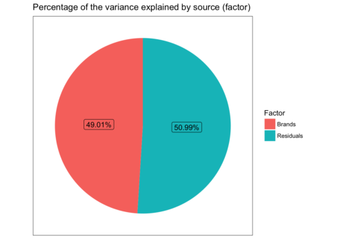
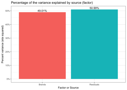
Probably more than needed for a simple Oneway but as a gateway to looking at more complex results in the future we can graph \(\eta^2\) as well. First we’ll use a pie to show relative contributions to variance. But since pie charts tend to be discouraged we’ll also do a bar graph.
The first step we need data to graph. As usual, I’ll try and get there with the fewest and simplest commands possible in R. If you remember above we used the etaSquared function from package lsr to get results. But ggplot2 prefers data frames. Rather than using something from base R or the tidyverse why don’t we simply coerce the results of our previous work into a data frame? I prefer to make the row.name into a neatly labelled column. The comments show you the same process skipping lsr and computing \(\eta^2\) on the fly.
dddd<-as.data.frame((etaSquared(tyres.aov,anova = TRUE)))
dddd$Factor<-row.names(dddd)
# dddd<-as.data.frame(anova(tyres.aov))
# dddd$Factor<-row.names(dddd)
# dddd$eta.sq<-dddd$`Sum Sq` / sum(dddd$`Sum Sq`)
Given this data frame we can start with a pie chart. To overcome any objection that humans can’t accurately divine the proportions I’ve labelled them. I will admit though that that’s quite a bit of code to make a pie chart.
ggplot(dddd, aes(x = 1,y= eta.sq,fill=Factor)) +
  geom_col() +
  geom_label(aes(
    label = scales::percent(eta.sq)),
    position = position_stack(vjust = 0.5),
    show.legend = FALSE) +
  coord_polar(theta='y') +
  theme_bw() +
  theme(axis.ticks=element_blank(),
        axis.title=element_blank(),
        panel.grid = element_blank(),
        axis.text.y=element_blank(),
        axis.text.x=element_blank()) +
  ggtitle("Percentage of the variance explained by source (factor)")

## Simple bar with percents
ggplot(dddd, aes(x = Factor,y= eta.sq,fill=Factor)) +
  geom_col() +
  geom_text(aes(y = eta.sq, label = scales::percent(eta.sq)), vjust = -0.25) +
  scale_y_continuous(labels = scales::percent) +
  ggtitle("Percentage of the variance explained by source (factor)") +
  ylab("Percent variance (eta squared)") +
  xlab("Factor or Source") +
  guides(fill=FALSE) +
  theme_bw()
We now know that we have significant test results both from the overall omnibus test and that 5 of the 6 pairs are significantly different. We have a good sense of how strong the relationship is between Brand and Mileage via the amount of the variance explained. But, before we close out our efforts we would do well to check our statistical assumptions.
Checking our assumptions
Most statistical tests results rest on meeting certain assumptions when we run the test. A Oneway ANOVA is no exception. We have assumed 3 things; independence, homogeneity of variance (homoscedasticity) and normality. We should see to these assumptions before we use or publish our results. Independence doesn’t have a simple answer in this case. The direct threat would be if there were some undisclosed/unknown dependence (for example two of the brands were manufactured in the same plant using the same equipment and simply branded differently). For now there doesn’t seem to be any reason to believe that we have violated this assumption.
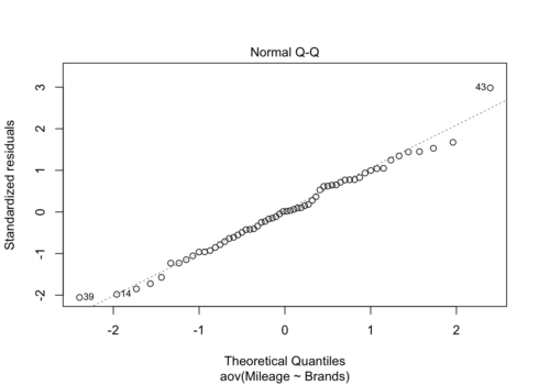
Next let’s address the assumption that our errors or residuals are normally distributed. We’re looking for evidence that our residuals are skewed or tailed or otherwise misshapen in a way that would influence our results. Surprisingly, there is actually quite a bit of controversy on this point since on the one hand we have strong reason to believe that our sample will be imperfect and that our population will not necessarily be “perfectly normal” either. Some argue that some simple plotting is all that is necessary looking for an unspecifiable amount of non normality that will trigger a search for the source. Other prefer a more formal approach using one or more statistical tests. We’ll address both.
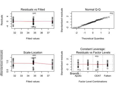
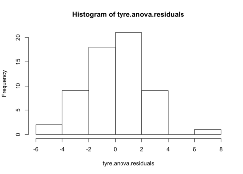
First we can plot the residuals using either a QQ plot or a histogram of the residuals themselves. In R we’ll code this as:
# Plot each one by one
plot(tyres.aov)
par(mfrow=c(2,2))
plot(tyres.aov)
par(mfrow=c(1,1))

# let's grab the residuals from our model
tyre.anova.residuals <- residuals( object = tyres.aov ) # extract the residuals
# A simple histogram
hist( x = tyre.anova.residuals ) # another way of seeing them
Nothing in these plots indicates we have a major violation. We can confirm that to some degree numerically by simply describing the residuals (describe command results). Let’s also run the two most common tests of the normality assumption (as usual there are others). First the Shapiro-Wilk test and then the Kolmogorov-Smirnov test (against a normal distribution). The summary statistics look good, low skew and kurtosis. The Shapiro-Wilks is simple to run. Feed it our residuals and it answers. Kolmogorov-Smirnov is a little more difficult to set up. It has many more potential uses so we have to feed it not just our data but also the fact that we are comparing to a theoretically cumulative normal distribution with our mean and our standard deviation.
describe(tyre.anova.residuals)
##    vars  n mean   sd median trimmed  mad   min  max range skew kurtosis   se
## X1    1 60    0 2.13   0.03       0 2.23 -4.33 6.29 10.62 0.15    -0.01 0.27
shapiro.test( x = tyre.anova.residuals ) # run Shapiro-Wilk test
##
##  Shapiro-Wilk normality test
##
## data:  tyre.anova.residuals
## W = 0.9872, p-value = 0.7826
ks.test(tyre.anova.residuals, "pnorm", mean(tyre.anova.residuals), sd(tyre.anova.residuals) )
##
##  One-sample Kolmogorov-Smirnov test
##
## data:  tyre.anova.residuals
## D = 0.062101, p-value = 0.9637
## alternative hypothesis: two-sided
The results are opposite of our usual thinking. Usually we would like to reject the null hypothesis. In this case we are glad to see that we can not reject the null. While it doesn’t prove “normality” (you can’t “prove” the null) it does allow us to say we have no reason to suspect our data are significantly non normal.
That’s two of three assumptions checked. The final is homogeneity of variance also known as (homoscedasticity). Since the math in our tests rely on the assumption that the variance for the different brands of tires is more or less equal. We need to check that assumption. I’ll tell you about what to do if it isn’t in a succeeding section.
In his post Professor Ghosh shows the Levene and Bartlett tests. Let’s replicate those and also visit a nuance about the Brown Forsyth test as well. All three tests help us test whether the variances amongst the groups are significantly different. Bartlett is the oldest and most complex mathematically and is sensitive to violations of normality. Levene tests using differences from the mean and Brown Forsyth differences from the median (making it more robust). When you run the leveneTest in R the default is actually a Brown Forsyth to get a true Levene you must specify center = mean.
leveneTest(tyres.aov, center = mean) # traditional Levene
## Levene's Test for Homogeneity of Variance (center = mean)
##       Df F value Pr(>F)
## group  3  0.6878 0.5633
##       56
leveneTest(tyres.aov) # technically a Brown Forsyth
## Levene's Test for Homogeneity of Variance (center = median)
##       Df F value Pr(>F)
## group  3  0.6946 0.5592
##       56
bartlett.test(Mileage~Brands,tyre) # yet another way of testing
##
##  Bartlett test of homogeneity of variances
##
## data:  Mileage by Brands
## Bartlett's K-squared = 2.1496, df = 3, p-value = 0.5419
Happily all the results are similar. We can not reject the null therefore we have no reason to question our assumption. The data have been good to us so far. But what should we do if we start having concerns about violating assumptions?
One of the common cases, for example, is just failing to have homogeneity of variance across our factor levels (in this case tire brand). There is a special variation of the ANOVA as well as the t test which allows us to drop the assumption and run the test. If you’ve never seen one you will be surprised that the degrees of freedom may be a decimal and likely quite different from your original. To use it we simply use oneway.test(Mileage ~ Brands, tyre) instead of our original aov(Mileage~Brands, tyre) the one downside is that it does not provide the full classic ANOVA table. It only tests the hypothesis and returns the results.
So in the code below I’ve run the Welch’s, then used oneway.test to run a classic ANOVA with var.equal = TRUE and finally for your convenience a summary of the original.
oneway.test(Mileage ~ Brands, tyre)
##
##  One-way analysis of means (not assuming equal variances)
##
## data:  Mileage and Brands
## F = 21.686, num df = 3.000, denom df = 30.773, p-value = 9.72e-08
# versus this which is what we've done so far
oneway.test(Mileage ~ Brands, tyre, var.equal = TRUE)
##
##  One-way analysis of means
##
## data:  Mileage and Brands
## F = 17.942, num df = 3, denom df = 56, p-value = 2.781e-08
# versus our original
summary(tyres.aov)
##             Df Sum Sq Mean Sq F value   Pr(>F)
## Brands       3  256.3   85.43   17.94 2.78e-08 ***
## Residuals   56  266.6    4.76
## ---
## Signif. codes:  0 '***' 0.001 '**' 0.01 '*' 0.05 '.' 0.1 ' ' 1
Other (Non-parametric) options?
Of course if you really want to be cautious about all of your assumptions (normality and homoscedasticity) then the non-parametric Kruskal-Wallis rank sum test is the way to go. As the name implies it uses ranks for the dependent variable mileage rather than the number of miles itself. What the test essentially does is test the hypothesis that all the group medians are equal. That is the equivalent omnibus test to a traditional Oneway ANOVA. The Dunn test is the analog to the post hoc pairwise comparisons we ran earlier. I’ve shown both separately but conveniently R reports both if you just run the second command.
kruskal.test(Mileage~Brands,tyre)
##
##  Kruskal-Wallis rank sum test
##
## data:  Mileage by Brands
## Kruskal-Wallis chi-squared = 29.733, df = 3, p-value = 1.57e-06
dunn.test(tyre$Mileage,tyre$Brands,method = "holm",alpha = 0.01)
##   Kruskal-Wallis rank sum test
##
## data: x and group
## Kruskal-Wallis chi-squared = 29.7331, df = 3, p-value = 0
##
##
##                            Comparison of x by group
##                                     (Holm)
## Col Mean-|
## Row Mean |     Apollo   Bridgest       CEAT
## ---------+---------------------------------
## Bridgest |   2.655358
##          |     0.0119
##          |
##     CEAT |   0.156812  -2.498546
##          |     0.4377     0.0125
##          |
##   Falken |  -2.791262  -5.446621  -2.948075
##          |     0.0105    0.0000*     0.0080
Clearly we can continue to reject the overall null hypothesis that the brand populations are all equal. But notice that the Dunn test does NOT support the conclusion that 5 out of 6 pairings are different at \(\alpha\) = 0.01. Clearly everything is tantalizingly close and if we were to run the test with the more traditional \(\alpha\) = 0.05 we’re fine right?
Well not exactly and that’s the last thing we’ll cover.
Plot twist – A Bayesian perspective
So up until now we have approaching our work from a strictly frequentist approach (for a great discussion of what that means see LSR pp 555 (and specifically starting at page 581 for ANOVA).
That means we have to be very careful to not talk about our tests returning probabilities (as opposed to setting decision boundaries). Briefly Bayesian methods allow us to calculate the probability or the odds that the mean mileage for Brands is different. If that’s what you’d really like to know in this case please read on.
If we choose a Bayesian approach to our research question we will wind up with something called a Bayes Factor (how original right?). If the Bayes Factor is for example 5 we would say that the odds are 5:1 in favor of the hypothesis that Brands matter. Quite useful if you ask me. We’d need some guidance on how to interpret how strong the odds are (in words) and Kass and Raftery (1995) {quoted in LSR} have provided those:
| Bayes factor | Interpretation | |
|---|---|---|
| 1 – 3 | Negligible evidence | . |
| 3 – 20 | Positive evidence | |
| 20 – 150 | Strong evidence | |
| 150 and above | Very strong evidence |
These seem pretty reasonable. What do we get for a Bayes Factor from our data? The BayesFactor package will tell us. The commands look very similar to what we used earlier.
tyres.bf.aov<- anovaBF(Mileage~Brands, tyre)
summary(tyres.bf.aov)
## Bayes factor analysis
## --------------
## [1] Brands : 435470.5 ±0%
##
## Against denominator:
##   Intercept only
## ---
## Bayes factor type: BFlinearModel, JZS
The odds are enormous that brand has an effect on mileage 435,470:1 and that’s a nice statement to be able to make. While covering the Bayesian approach is well beyond this tutorial I do encourage folks to have a look.
I hope you’ve found this useful. I simply built on another’s work and am open to comments, corrections and suggestions.
You can find the full code and RMarkdown file here.
