With the BMuCaret Shiny app post you can perform Caret-models comparison and find the best one, which achieves the best performance for a given data set.
But isn't it true that “All models are wrong”?
By conducting comparison of predictive models (e.g. by using my tool BMuCaret) the goal of this experience is not to find a model, which is exactly true, but to find the best one which describes better the problem we are studying (in my example, I let the model estimate the probability that a customer will churn).
In general, when building statistical models, we must not forget that the aim is to understand something about the real world. Or predict, choose an action, make a decision, summarize evidence, and so on, but always about the real world, not an abstract mathematical world: our models are not the reality—a point well made by George Box in his oft-cited remark that “ all models are wrong, but some are useful”. Notes from here and here
Usability of predictive models
To make the selected predictive model interpretable and therefore useful for user I think the most important thing to do first is extracting the information necessary – such variable importance, variable effects, the relationship between variables and the model output …- to examine and understand the learned model.
In the context of machine learning interpretability is defined
as the ability to explain or to present in understandable terms to a human.
… we argue that interpretability can assist in qualitatively ascertaining whether other desiderata—such as fairness, privacy, reliability, robustness, causality, usability, and trust—are met.
Towards A Rigorous Science of Interpretable Machine Learning
If you understand how your model produces predictions:
- you will be better equipped to improve it
- you can explain your model to user
- your model will then assist user to accomplish tasks-e.g. produce customer-level models that describe the likelihood that a customer will take a particular action/develop an action plan to reduce customer churn
Post-hoc explanation tools
There are several methods and tools that can be used to conduct post-hoc explanation and let people understand why the system works the way it does:
- LIME(Local Interpretable Model-Agnostic Explanations): is a method for explaining the outcome of black box models by fitting a local model around the point in question an perturbations of this point. Description
- breakDown: Model agnostic tool for decomposition of predictions from black boxes.Break Down Table shows contributions of every variable to a final prediction. Break Down Plot presents variable contributions in a concise graphical way. This package work for binary classifiers and general regression models. Description
- DALEX (Descriptive mAchine Learning EXplanations): Dalex package contains various explainers that help to understand the link between input variables and model output. Description
- IML(Interpretable Machine Learning): interpretability methods to analyze the behavior and predictions of any machine learning model. Description
New function in BMuCaret App.: post-hoc model explanation
New functionalities have been implemented in my BMuCaret shiny App., which will assist you in an easy way (just some klicks) to conduct a post-hoch explanation of predictive models (candidate models: eXtreme Gradient Boosting, glmnet, LDA, Neural Network, Random Forest).
IML and DALEX packages have been used to implement these functionalities.
More on IML Package here and About DALEX here
Implemmented technics for conducting post hoch explanation
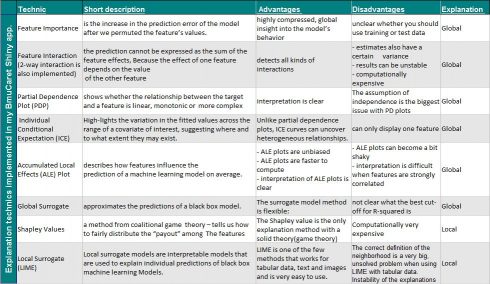
The implemented tools/technics in BMuCaret for analyzing machine learning model on Dataset-Level (Global explanation) and on Prediction Level (local explanation) are listed in the table below.
A detailed description can be found in Interpretable Machine Learning, A Guide for Making Black Box Models Explainable.Author: Christoph Molnar, also founder of the IML package
Some Examples
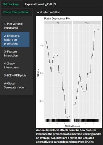
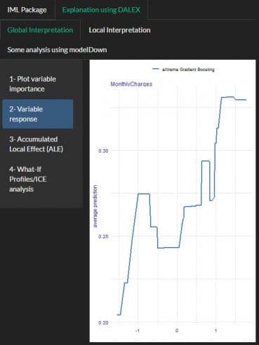
PDP using IML and DALEX:
A partial dependence plot can show whether the relationship between the target and a feature is linear, monotonic or more complex
Using IML package
Using DALEX package
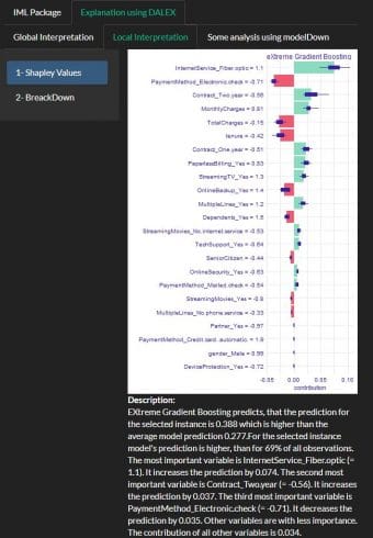
Example Sharpley values using DALEX
A prediction can be explained by assuming that each feature value of the instance is a “player” in a game where the prediction is the payout. Shapley values – a method from coalitional game theory – tells us how to fairly distribute the “payout” among the features.
The SHAP values plot shows also the positive and negative relationships of the variables with the target variable (Churn).
I did use the function describe{iBreakDown} to generate natural language explanations (Description at the bottom of the plot).
BMuCaret Code
The code for BMuCaret application consists of 4 Modules:
- Module1: Load needed packages and the data set in scope
- Module2: pre-Processing the data using recipe
- Module3: Construct model grid and define shared settings
- Module4: The code for the Shiny application. This module has been updated with post hoch explanation functionalities.
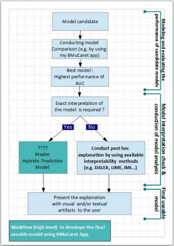
The following diagram is giving a high-level overview of the workflow for developing the final best and usable predictive Caret models.
Conclusion and outlook
With the updated BMuCaret Shiny application, you can not only perform modeling and find the best Caret model for your predictive problem but also generate explanations for the predictions of your trained black-box classifier (Caret models).
All the implemented explanation technics are useful tools to provide insight into the internal decision-making process of the algorithm used, however, they do not exactly characterize the decision-making process and
they cannot have perfect fidelity with respect to the original model. If the explanation was completely faithful to what the original model computes, the explanation would equal the original model, and one would not need the original model in the first place, only the explanation. (In other words, this is a case where the original model would be interpretable.) This leads to the danger that any explanation
method for a black-box model can be an inaccurate representation of the original model in parts of the feature space more here.
In working in high stakes decisions field one should be very careful when applying post hoc methods with unknown descriptive accuracy. Please Stop Explaining Black-Box Models for High Stakes Decisions this is a must-read!
Hybrid Predictive Model could be an alternative solution:
A hybrid predictive model is not a pure interpretable model. It utilizes the partial predictive power of black-box models to preserve the predictive accuracy. It is also not an explainer model which only observes but does not participate in the decision process. Here, a hybrid predictive model uses an interpretable model and a black-box model jointly to make a prediction more here.
This novel framework for learning a Hybrid Predictive Model is promising and it will be very likely the subject of my next blog post.
And here is the code:
#################################### Module1: Load needed packages and the data set in scope ########
library(shiny)
library(shinyBS)
library(shinythemes)
library(modelgrid)
library(magrittr)
library(caret)
library(e1071)
library(foreach)
library(recipes)
library(purrr)
library(dplyr)
library(pROC)
library(BradleyTerry2)
library(corrplot)
library(DataExplorer)
library(randomForest)
library(glmnet)
library(xgboost)
library(readr)
library(ggplot2)
library(mlbench)
library(e1071)
library(DALEX)
library(pdp)
library(ICEbox)
library(iml)
library(ingredients)
library(iBreakDown)

####################
# load data
set.seed(9650)
Telco_customer_3 <- read.csv("D:/Quellen/Telecom customer/WA_Fn-UseC_-Telco-Customer-Churn.csv")
data_set <- Telco_customer_3
data_set <- data_set%>%dplyr::select(-"customerID")
data_set$Churn <- as.factor(data_set$Churn)
######################## Module2:  pre-Processing the data using recipe
set.seed(9650)
Attri_rec_2 <-
    recipe(Churn ~ ., data = data_set) %>%        # Formula.
    step_dummy(all_predictors())%>%               # convert nominal data into one or more numeric.
    step_knnimpute(all_predictors())%>%           # impute missing data using nearest neighbors.
    step_zv(all_predictors()) %>%                 # remove variables that are highly sparse and unbalanced.
    step_corr(all_predictors()) %>%               # remove variables that have large absolute correlations with other variables.
    step_center(all_predictors()) %>%             # normalize numeric data to have a mean of zero.
    step_scale(all_predictors()) %>%              # normalize numeric data to have a standard deviation of one.
    prep(training = data_set, retain = TRUE)      # train the data recipe

data_rec_2 <- as.data.frame(juice(Attri_rec_2))
# add the response variable
data_rec_2$Churn <- data_set$Churn
# str(data_rec_2)
# Create a Validation Dataset (training data 70% and validation data 30% of the original data)
set.seed(9650)
validation_index <- createDataPartition(data_rec_2$Churn,times= 1,  p= 0.70, list=FALSE)
# select 30% of the data for validation
data_validation <- data_rec_2[-validation_index,]
# use the remaining 70% of data to train the models
data_train <- data_rec_2[validation_index, ]
# For traing the models
x_train <- data_train%>%select(-Churn) # Predictors
y_train <- data_train[["Churn"]] # Response
# for validation/test
x_validation <- data_validation%>%select(-Churn)
y_validation <- data_validation[["Churn"]]
## Vaiable list
variable_list <- colnames(x_validation)

##############  Module 3 Construct model grid and define shared settings.####################
set.seed(9650)
mg <-
    model_grid() %>%
    share_settings(
        y = y_train,
        x = x_train,
        metric = "ROC",
        trControl = trainControl(
            method = "adaptive_cv",
            number = 10, repeats = 5,
            adaptive = list(min =3, alpha =0.05, method = "BT", complete = FALSE),
            search = "random",
            summaryFunction = twoClassSummary,
            classProbs = TRUE))
purrr::map_chr(mg$shared_settings, class)
## add models to train
mg_final <- mg %>%

  add_model(model_name = "LDA",
              method = "lda",
              custom_control = list(method = "repeatedcv",
                                    number = 10,
                                    repeats =5))%>%
  add_model(model_name = "eXtreme Gradient Boosting",method = "xgbDART")%>%
  add_model(model_name = "Neural Network", method = "nnet")%>%
  add_model(model_name = "glmnet", method = "glmnet")%>%
  add_model(model_name = "Random Forest", method = "rf")
#%>% add_model(model_name = "gbm",
# method="gbm", custom_control = list(verbose = FALSE))

list_model <- c(names(mg_final$models))

################################# Module4: Shiny application #########################
ui <- fluidPage(theme = shinytheme("darkly"),
## Application title
      titlePanel(wellPanel("Model Explanation with BMuCaret Shiny Application",br(),"BMuCaret2")),
        navbarPage("Workflow ===>",
           tabPanel("Exploratory Data Analysis",
              tabsetPanel(type = "tabs",
              tabPanel("Explore the data object",
                 navlistPanel(
                   tabPanel("1- Structure of the data object", verbatimTextOutput("str_ucture")),
                   tabPanel("2- Missing values ?", plotOutput("missing_value")),
                   tabPanel("3- Correlation analysis", plotOutput("coor_plot", height = 700)))),
              tabPanel("After Data Cleaning (using recipe method)",
                navlistPanel(
                  tabPanel("1- Structure of the data object after Processing",
                           verbatimTextOutput("str_ucture_after")),
                  tabPanel("2- Missing values ?", plotOutput("missing_value_after") ),
                  tabPanel("3- Correlation analysis after", plotOutput("coor_plot_after", height = 600))                                                         )))),
              tabPanel("Fitting & Validation & Statistics",
                sidebarLayout(
                  sidebarPanel(
                    wellPanel(selectInput(inputId = "abd",
                      label = "Model choose : ",
                      choices = c("none", list_model),
                      selected = "none", width = '200px'))),
        mainPanel(
          tabsetPanel(type= "tabs",
## output model training and summary
            tabPanel("Model Training & Summary",
             navlistPanel(
               tabPanel("1- Show info model grid ",verbatimTextOutput("info_modelgrid")),
               tabPanel("2- Performance statistics of the model grid (dotplot) ",
                        plotOutput("dotplot", width = 600, height = 600)),
               tabPanel("3- Extract Performance of the model grid ", verbatimTextOutput(outputId = "summary")),
               tabPanel("4- Show the AUC & Accuracy of individual models (on data training)",
                    verbatimTextOutput("Accurac_AUC"), htmlOutput("best_model_train")),
               tabPanel("5- Show Statistics of individual model", verbatimTextOutput(outputId = "Indiv_Analysis")
                      ,"Examine the relationship between the estimates of performance
                      and the tuning parameters", br(),
                      plotOutput(outputId= "tuning_parameter")),
               tabPanel("6- Show single model's Accuracy (on data training)",
                        verbatimTextOutput(outputId = "accuracy")))),
## output model validation and statistics
          tabPanel("Model Validation & Statistics",
           navlistPanel(
             tabPanel("1-Show the AUC & Accuracy of individual models (on validation data)",
                    verbatimTextOutput(outputId = "AUC_of_individ"), htmlOutput("best_model_vali")),
            tabPanel("2- Show single model's Accuracy/data validation",
                     verbatimTextOutput("accuracy_vali"))))

    )))),
  ###########################################################  Module post hoch explanation ################
      tabPanel("Model Explanation",
        sidebarLayout(
          sidebarPanel(
            wellPanel(selectInput(inputId = "perf",
                                  label = "Model choose : ",
                                  choices = c("none", list_model),
                                  selected = "none", width = '200px')),

            wellPanel(selectInput(inputId = "Variab_le",
                                  label = "Variable choose : ",
                                  choices = c("none", variable_list),
                                  selected = "none", width =  '200px')),
            wellPanel(numericInput(inputId="row_index",
                                   label= "Insert the row number",
                                    value=1,
                                    min=1, max=20,  width = '200px'))),
        mainPanel(
          tabsetPanel(type = "tabs",
  #### IML Packge#######
           tabPanel("IML Package",
            tabsetPanel(type = "tabs",
              tabPanel("Global Interpretation",
                navlistPanel(
                 tabPanel("1- Plot variable importance", plotOutput("variable_imp", height = "600px"),
                              verbatimTextOutput("condition")),
                 tabPanel("2- Effect of a feature on predictions",
                              plotOutput("PD_P", height = "600px"), htmlOutput("des")),
                 tabPanel("3- Feature Interaction", plotOutput("inter_action", height = "600px")),
                 tabPanel("4- 2-way interactions", plotOutput("two_way_inter", height = "600px"),
                              verbatimTextOutput("condition2")),
                 tabPanel("5- ICE + PDP plots", plotOutput("IC_E")),
                 tabPanel("6- Global Surrogate model",
                              plotOutput("surrogate_model", height = "600px")))),
                 tabPanel("Local Interpretation",
                   navlistPanel(
                    tabPanel("1- Shapley Values", plotOutput(outputId = "shapley_Values", height = "600px")),
                    tabPanel("2- LIME", plotOutput(outputId = "single_plot_lime", height = "600px")))))),
      #### DALEX Packge#######
              tabPanel("DALEX Package",
                tabsetPanel(type = "tabs",
                  tabPanel("Global Interpretation ",
                    navlistPanel(
                      tabPanel("1- Plot variable importance",
                                     plotOutput("variable_imp_da", height = "600px"),
                                     verbatimTextOutput("condition_da")),
                      tabPanel("2- Variable response", plotOutput("Vari_resp", height = "600px")),
                      tabPanel("3- Accumulated Local Effect (ALE)", plotOutput("ALE_da"),
                                     verbatimTextOutput("condition2_da")),
                      tabPanel("4- What-If Profiles/ICE analysis ",
                                     plotOutput("what_if", height = "600px")))),

                      tabPanel("Local Interpretation ",
                       navlistPanel(
                        tabPanel("1- Shapley Values", plotOutput(outputId = "shapley_Values_da", height = "600px"),
                                   htmlOutput("descri_ption_sharp")),
                        tabPanel("2- BreackDown", plotOutput(outputId = "single_plot_brd_da",
                                                               height = "600px"),htmlOutput("descri_ption")))),
                        tabPanel("Some analysis using modelDown ", br(), br(),
                                   actionButton("do", "Click here to generate a website with HTML
                                   to get summary: auditor, drifter, model_performance,
                                                variable_importance, and variable_response", width = '90px' ))))
                    ))))),
############ Contact #############
 br(), br(),br(),
  h5("BMuCaret App. built with", img(src =
    "https://d33wubrfki0l68.cloudfront.net/8f68bc526580587d60714f9279fbe9d86b25362a/79958/assets/img/shiny.png",
    height= "30px"),
   "by",
  br(),
  "Author: Abderrahim Lyoubi-Idrissi",
  br(),
 "Contact: kritiker2017@gmail.com")
)

################################# Define server logic #########################

server <- function(input, output, session) {

    set.seed(9650)
    # before processing the data
    # data structure
    output$str_ucture <- renderPrint({
        str(data_set)
    })

## Missing values ?
    output$missing_value <- renderPlot({
        plot_missing(data_set)
    })
    # plot to check the results of step_corr(all_predictors())

    output$coor_plot <- renderPlot({
        plot_correlation(data_set)
    })

## after processing the data
  # data structure
    output$str_ucture_after <- renderPrint({
        str(data_rec_2)
    })
    # plot to check the missing values
    output$missing_value_after <- renderPlot({
        plot_missing(data_rec_2)
    })
    # plot to check the correlation
    output$coor_plot_after <- renderPlot({
        plot_correlation(data_rec_2)
    })
    set.seed(9650)
## Infos about the componets of the constructed model grid
    output$info_modelgrid <- renderPrint({
        mg_final$models
    })
## train all models
    set.seed(9650)
    mg_final_tra <- reactive({train(mg_final)})
    ## plot to compare
    output$dotplot <- renderPlot({
        mg_final_tra()$model_fits %>%
            caret::resamples(.) %>%
            lattice::dotplot(.)
    })
## Show the overall summary
    set.seed(9650)
    output$summary <- renderPrint({
        mg_final_tra()$model_fits %>%
            caret::resamples(.) %>%
            summary(.)
    })

## computing the auc & the accuracy (on train data)
    set.seed(9650)
    output$Accurac_AUC <- renderPrint({
        AUC1 <- mg_final_tra()$model_fits%>% predict(., newdata = x_train, type ="prob")%>%
          map(~roc(y_train, .x[,2]))
        auc_value_train <- map_dbl(AUC1, ~(.x)$auc)
        auc_value_df_train_df <- as.data.frame(auc_value_train)
        accuarcy_all_train <- predict(mg_final_tra()$model_fits, newdata = x_train)%>%
          map( ~confusionMatrix(.x, y_train))%>%
            map_dfr(~ cbind(as.data.frame(t(.x$overall)),as.data.frame(t(.x$byClass))), .id = "Modelname")%>%
            select(Modelname, Accuracy, Kappa)
        accuracy_auc_train <-  bind_cols(accuarcy_all_train, auc_value_df_train_df)
        accuracy_auc_train
     })
## computing the auc and the Accuracy
    set.seed(9650)
    output$best_model_train <- renderUI({

        AUC1 <- mg_final_tra()$model_fits%>% predict(., newdata = x_train, type ="prob")%>%
            map(~roc(y_train, .x[,2]))

        auc_value_train <- map_dbl(AUC1, ~(.x)$auc)
        auc_value_df_train_df <- as.data.frame(auc_value_train)

        accuarcy_all_train <- predict(mg_final_tra()$model_fits, newdata = x_train)%>%
            map( ~confusionMatrix(.x, y_train))%>%
            map_dfr(~ cbind(as.data.frame(t(.x$overall)),as.data.frame(t(.x$byClass))), .id = "Modelname")%>%
            select(Modelname, Accuracy, Kappa)

        accuracy_auc_train <-  bind_cols(accuarcy_all_train, auc_value_df_train_df)

        max_auc_train <- filter(accuracy_auc_train, auc_value_train == max(accuracy_auc_train$auc_value_train))%>%
            select(Modelname)
        max_Accuracy_train <- filter(accuracy_auc_train, Accuracy == max(accuracy_auc_train$Accuracy))%>%
            select(Modelname)

        HTML(paste("Results", br(),
                   "1- The model", strong(max_auc_train), "has the highest AUC value.", br(),
                   "2- The model",strong(max_Accuracy_train), "has the highest Accuracy" ))
    })
    # Show the summary of individual model
    output$Indiv_Analysis <- renderPrint({if(input$abd == "none"){print("Please select a model")}
        mg_final_tra()$model_fits[[input$abd]]
    })
    # Plot the individual model
    output$tuning_parameter <- renderPlot({
        ggplot( mg_final_tra()$model_fits[[input$abd]])
    })

    # ConfusionMatrix on training data
    output$accuracy <- renderPrint({if(input$abd == "none"){print("Please select a model")}
        else{ confusionMatrix( predict(mg_final_tra()$model_fits[[input$abd]], x_train), y_train)}
    })

   ########################### Model Validation #########################
# Extract the auc values
    output$AUC_of_individ <- renderPrint({
        AUC2 <- mg_final_tra()$model_fits%>% predict(., newdata = x_validation, type ="prob")%>%
            map(~roc(y_validation, .x[,2]))

        auc_value_vali <- map_dbl(AUC2, ~(.x)$auc)
        auc_value_df_vali_df <- as.data.frame(auc_value_vali)

        cf_vali <- predict(mg_final_tra()$model_fits, newdata = x_validation)%>%
            map( ~confusionMatrix(.x, y_validation))
        cf_vali%>%
            map_dfr(~ cbind(as.data.frame(t(.x$overall)),as.data.frame(t(.x$byClass))), .id = "Modelname")%>%
            select(Modelname, Accuracy, Kappa)

        accuarcy_all_vali <- predict(mg_final_tra()$model_fits, newdata = x_validation)%>%
            map( ~confusionMatrix(.x, y_validation))%>%
            map_dfr(~ cbind(as.data.frame(t(.x$overall)),as.data.frame(t(.x$byClass))), .id = "Modelname")%>%
            select(Modelname, Accuracy, Kappa)
        accuracy_auc_vali <-  bind_cols(accuarcy_all_vali,auc_value_df_vali_df)
        print(accuracy_auc_vali)
     })

    output$best_model_vali <- renderUI({

        AUC2 <- mg_final_tra()$model_fits%>%
            predict(., newdata = x_validation, type ="prob")%>%
            map(~roc(y_validation, .x[,2]))

        auc_value_vali <- map_dbl(AUC2, ~(.x)$auc)
        auc_value_df_vali_df <- as.data.frame(auc_value_vali)

        cf_vali <- predict(mg_final_tra()$model_fits, newdata = x_validation)%>%
            map( ~confusionMatrix(.x, y_validation))
        cf_vali%>%
            map_dfr(~ cbind(as.data.frame(t(.x$overall)),as.data.frame(t(.x$byClass))), .id = "Modelname")%>%
            select(Modelname, Accuracy, Kappa)

        accuarcy_all_vali <- predict(mg_final_tra()$model_fits, newdata = x_validation)%>%
            map( ~confusionMatrix(.x, y_validation))%>%
            map_dfr(~ cbind(as.data.frame(t(.x$overall)),as.data.frame(t(.x$byClass))), .id = "Modelname")%>%
            select(Modelname, Accuracy, Kappa)

        accuracy_auc_vali <-  bind_cols(accuarcy_all_vali,auc_value_df_vali_df)

        max_auc_vali <- filter(accuracy_auc_vali, auc_value_vali == max(accuracy_auc_vali$auc_value_vali))%>%
            select(Modelname)
        max_Accuracy_vali <- filter(accuracy_auc_vali, Accuracy == max(accuracy_auc_vali$Accuracy))%>%
            select(Modelname)


        HTML(paste("Results", br(),
                   "1- The model", strong(max_auc_vali), "has the highest AUC value.", br(),
                   "2- The model",strong(max_Accuracy_vali), "has the highest Accuracy."))
     })

## confusion matrix on data validation
    output$accuracy_vali<- renderPrint({if(input$abd == "none"){print("Please select a model")}
        else{
            confusionMatrix(predict(mg_final_tra()$model_fits[[input$abd]], x_validation), y_validation)}
     })

############################## Model explaination  #######################################
  ############## Using IML Package ###################################
## define the IML predictor
  mod2 <- reactive({ Predictor$new(mg_final_tra()$model_fits[[input$perf]],
                        data = x_validation, y= y_validation,  type = "prob")})

## plot the variable importance
    output$condition <- renderPrint({
      if(input$perf == "none"){print("Please select a model")}
      else{

      output$variable_imp <- renderPlot({
      vari_imp <- FeatureImp$new(mod2(), loss = "ce")
      plot(vari_imp)})
      }})
## Visualise the features interaction
    output$inter_action <- renderPlot({
      plot(Interaction$new(mod2()))
      })

    output$condition2 <- renderPrint({
      if(input$Variab_le == "none"){print("Please select a variable")}
      else{
      output$two_way_inter <- renderPlot({
    plot(Interaction$new(mod2(), feature = input$Variab_le)) })}
      })

## Feature effects
    output$PD_P <-  renderPlot({
      ale <- FeatureEffect$new(mod2(), feature = input$Variab_le)
      plot(ale) +
        ggtitle("Partial Dependence Plot")
      })

    output$des <- renderUI({
      br()
      HTML(paste(
        strong("Accumulated local effects describe how features influence the prediction
        of a machine learning model on average. ALE plots
        are a faster and unbiased alternative to partial dependence Plots (PDPs).")))
     })

## Plot PDP and ICE
   output$IC_E <- renderPlot({
        plot(FeatureEffect$new(mod2(), feature = input$Variab_le, method = "pdp+ice"))
    })

## Surrogate model
   output$surrogate_model <- renderPlot({
     tree <-  TreeSurrogate$new(mod2(), maxdepth = 2)
     plot(tree)
   })

## Shapley Values
  # Explain single predictions with game theory

  output$shapley_Values <- renderPlot({
   shapley <- reactive ({Shapley$new(mod2(), x.interest = x_validation[input$row_index, ])})
   plot(shapley())

  })

## LIME
  # Explain single prediction with LIME

 output$single_plot_lime <- renderPlot({

   lime.explain = LocalModel$new(mod2(),x.interest = x_validation[input$row_index,])
   lime.explain$results %>%
     ggplot(aes(x = reorder(feature.value, -effect), y = effect, fill = .class)) +
     facet_wrap(~ .class, ncol = 1) +
     geom_bar(stat = "identity", alpha = 1) +
     scale_fill_discrete() +
     coord_flip() +
     labs(title = paste0("Instance row number: ", input$row_index)) +
     guides(fill = FALSE)
 })

  ############## using DALEX Package  ###################################
## definde DALEX explainer
y_validation_da <- factor(ifelse(y_validation == "Yes", 1, 0))
yTest = as.numeric(as.character(y_validation_da))
p_fun <- function(object, newdata){predict(object, newdata= newdata, type="prob")[,2]}

explainer_da <- reactive({ explain(mg_final_tra()$model_fits[[input$perf]], label = input$perf,
                                   data = x_validation, y= yTest,
                                   predict_function = p_fun)

 })
## plot  variable importance with DALEX
output$condition_da <- renderPrint({
   if(input$perf == "none"){print("Please select a model")}
   else{
     output$variable_imp_da <- renderPlot({
      vari_imp_da <-  feature_importance(explainer_da(), loss_function = loss_root_mean_square)
       plot(vari_imp_da)
     })
   }})

## PDP plot
output$Vari_resp <- renderPlot({
 Vari_response <- ingredients::partial_dependency( explainer_da(), variables = input$Variab_le)
 plot(Vari_response)
})
## ALE plot
output$ALE_da <- renderPlot({
  accumulated_da <- accumulated_dependency( explainer_da(), variables = input$Variab_le)
  plot( accumulated_da)
})

## What if Profiles/ICE
output$what_if <- renderPlot({
 cp_model <- ceteris_paribus(explainer_da(), x_validation[input$row_index, ])
 plot(cp_model, variables = input$Variab_le) +
 show_observations(cp_model, variables = input$Variab_le) +
 ggtitle("Ceteris Paribus Profiles of the selected model")
})
## BreackDown Plot
output$single_plot_brd_da <- renderPlot({
  brd_da <- break_down(explainer_da(),
                                x_validation[input$row_index, ], keep_distributions = TRUE)
  plot(brd_da)
})
## Description
output$descri_ption <- renderUI({
  brd_da <- break_down(explainer_da(), x_validation[input$row_index, ],
                       keep_distributions = TRUE)
  br()
  HTML(paste(strong("Description:"),
             br(),
             describe(brd_da,
                      short_description = FALSE,
                      display_values =  TRUE,
                      display_numbers = TRUE,
                      display_distribution_details = FALSE)))
})

## Shapley Values
# Explain single predictions with game theory
output$shapley_Values_da <- renderPlot({
  shap_values <- shap(explainer_da(), x_validation[input$row_index, ], B=25)
  plot(shap_values)
 })

output$descri_ption_sharp <- renderUI({
     shap_values <- shap(explainer_da(), x_validation[input$row_index, ], B=25)
br()
HTML(paste(
      strong("Description:"),
              br(),
              describe(shap_values,
                       short_description = FALSE,
                       display_values =  TRUE,
                       display_numbers = TRUE,
                       display_distribution_details = FALSE)))
 })

## Generates a website with HTML summaries for the selected predictive model
observeEvent(input$do,
              {modelDown::modelDown( explainer_da())})

output$down_mod <- renderUI({HTML(paste("to summary: auditor, drifter, model_performance,
                                                variable_importance, and variable_response"))})

   ################################# Run the application #########################
}
shinyApp(ui = ui, server = server)
