If you measure the same person twice, you have longitudinal data. We all love longitudinal data because we can understand how their health outcomes change with time and this helps answering many interesting research questions. However, newer R users often face a problem in managing longitudinal data because it often comes in two ‘shapes’: the wide and the long. Some analysis can be easily conducted in wide format (e.g. two-sample t-tests) while the others require a long one (e.g. growth curve models). This article aims to provide you an overview of what long and wide format data are and how you could easily convert between them.
Let’s work with an example. Imagine you have a randomised controlled trial (RCT) for reducing people’s depression symptoms. The RCT have two treatments: Tx A and B. Each of the participants are measured three times: pre-intervention (time=1), immediate post-intervention (time=2), and a long-term follow up (time=3). You have a perfect situation where all the 500 participants (250 in Tx A and 250 in B) have completed all measurements.
We start with the wide data first.
In the imaginary RCT, the wide data will be a data frame with 500 rows, one row for each participants, and 4 columns storing the participant identifiers, the treatment allocation, and the three depression scores.
The first few rows of a wide data-set look like this:
subject.id tx measure.1 measure.2 measure.3
         1  A  27.61686  19.57415  24.10536
         2  A  41.46307  25.26103  32.82880
         3  A  33.97125  26.57679  42.66070
         4  A  31.03210  13.75620  23.50204
         5  A  28.27894  19.57316  27.29456
         6  A  37.97978  24.92336  30.52496
Data in long format looks much longer because each row represent one time-point. We have 500 participants, so the long data will have 500*3=1500 rows.
The first few rows of a long data-set look like this:
subject.id tx time  measure
         1  A    1 27.61686
         2  A    1 41.46307
         3  A    1 33.97125
         4  A    1 31.03210
         5  A    1 28.27894
         6  A    1 37.97978
Let’s start by converting a wide-formatted data into the long one.
The first part of the code is just for simulating a wide data-set for you. Don’t worry if you don’t understand them.
Generate a longitudinal dataset in wide-format
 #Generate a longitudinal dataset in wide-format
library(MASS)
dat.tx.a <- mvrnorm(n=250, mu=c(30, 20, 28),
                    Sigma=matrix(c(25.0, 17.5, 12.3,
                                   17.5, 25.0, 17.5,
                                   12.3, 17.5, 25.0), nrow=3, byrow=TRUE))
dat.tx.b <- mvrnorm(n=250, mu=c(30, 20, 22),
                    Sigma=matrix(c(25.0, 17.5, 12.3,
                                   17.5, 25.0, 17.5,
                                   12.3, 17.5, 25.0), nrow=3, byrow=TRUE))
dat <- data.frame(rbind(dat.tx.a, dat.tx.b))
names(dat) = c("measure.1", "measure.2", "measure.3")
dat <- data.frame(subject.id=factor(1:500), tx=rep(c("A", "B"), each=250), dat)
rm(dat.tx.a, dat.tx.b)
Putting all above codes in your R console (or R Studio), you’d have a data frame named dat. It has 500 rows (each for one participant) with five variables.
The dat data frame will look like this:
head(dat)
subject.id tx measure.1 measure.2 measure.3
         1  A  31.92417  15.56895  30.68700
         2  A  28.42165  25.89814  29.63313
         3  A  30.29753  18.39888  27.62321
         4  A  38.20373  30.37958  36.97875
         5  A  23.58534  12.63344  28.62889
         6  A  27.08170  14.49750  22.65016
Convert wide-formatted data into long
#Convert wide-formatted data into long
dat <- reshape(dat, varying=c("measure.1", "measure.2", "measure.3"),
               idvar="subject.id", direction="long")
Here we used the reshape() function. The first argument designates the data frame we want to convert. The second argument varying= designates the variables that are varied with time (which are the depression scores in this case). The third argument idvar= designates the participants’ identifiers. The fourth direction= designates the direction of conversion.
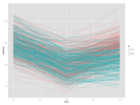
We have our data-set in long format now. To show you why we want the long data, we will plot the individual growth curves. The codes below make use of the powerful ggplot2 package which will be covered in the future tutorials.
Plot individual growth curves
#Plot individual growth curves
install.packages("ggplot2")
library(ggplot2)
ggplot(dat, aes(x=time, y=measure, colour=tx, group=subject.id)), geom_line(alpha=.5)
Don’t run the first line if you already have the package installed, as re-installing takes some time.
The end product will be like:

Although plotting growth curve is easier with long data, testing differences at a single time-point would be more convenient using a wide data-set. So we’d now convert the long data-set dat back into the wide format.
Convert long-formatted data into wide
#Convert long-formatted data into wide
dat <- reshape(dat, v.names="measure", timevar="time",
               idvar="subject.id", direction="wide")
Yes, we’re using the reshape() function again but this time we’re feeding different arguments. For converting long data into wide, we use v.names= to designate the time-varying variable. Please also note to use "wide" option for the direction= argument.
And finally we would be using the wide data for comparing the treatment difference:
# Testing the immediate post-intervention difference
with(dat, t.test(measure.2~tx))
In this line of code, we used with() function to tell R to look for the two variables measure.2 and tx inside the dat data-set. The t.test() function is a standard one for one-sample, paired, and two-sample t-tests. By assigning a formula-alike measure.2~tx argument into the function, R will assume it’s a two-sample t-test problem and calculate the result for us.
So here is the results:
Welch Two Sample t-test
data:  measure.2 by tx
t = -0.57703, df = 495.61, p-value = 0.5642
alternative hypothesis: true difference in means is not equal to 0
95 percent confidence interval:
 -1.120015  0.611492
sample estimates:
mean in group A mean in group B
       19.69917        19.95343
Ooops, no significant difference were detected at the immediate post-intervention measurement. But please don’t be disappointed because the story doesn’t end here.
This data needs a more in-depth analysis, and we would provide a walkthrough step-by-step.
Stay tuned.