For this post, I wanted to take the data analysis process in a different direction. Normally, an R analysis starts with data from a comma-separated Excel file (.csv) or a tab-separated file (.txt).
However, online data is often formatted in JSON, which stands for JavaScript Online Notation. JSON has different forms, but for this data, it consists of nested arrays in two main parts. One part is the meta-data header, and the other is the observations themselves. You can see that by looking at the file online here.
This data is LA city revenue, broken down by fiscal month and department. I want to get the total monthly revenue for the entire city and looks for seasonal trends.
To do this, we need to load in our JSON file, manipulate it, and apply time series analysis. Let’s get started.
JSON Manipulation
We load in the JSON file just as we would any other file type. However, R cannot read it, and that’s where “rjson” package comes into play. Once we extract the JSON file, we obtain the observations in the data section and create a variable for the number of observations.
#Install package
install.packages("rjson")
library(rjson)
jsonfile <- "yourpath/losangelesrevenue.json"

#Extract JSON data using rjson
rev <- fromJSON(txt=jsonfile)
datalength <- length(rev$data)
As I mentioned, let’s looks at the observations data, which is in arrays but can be manipulated like a matrix. We first create arrays to store the values, then loop over the arrays to get each value by its index. In JSON, we first get to the correct observation with the [[x]] parameter, then choose the value within the vector with the [9] parameter. We now have arrays for the fiscal year, month, department, revenue, and fiscal period.
datalength <- length(rev$data)

yeardata <- {}
monthdata <- {}
department <- {}
revenue <- {}
fiscalperiod <- {}

for (x in 1:datalength) {
  yeardata <- c(yeardata,as.integer(noquote(rev$data[[x]][9])))
  monthdata <- c(monthdata,toString(noquote(rev$data[[x]][10])))
  department <- c(department,toString(noquote(rev$data[[x]][12])))
  revenue <- c(revenue,as.double(noquote(rev$data[[x]][13])))
  fiscalperiod <- c(fiscalperiod,toString(noquote(rev$data[[x]][19])))
Data Frame Manipulation
First we need to combine our vectors into a data frame to combine monthly revenue.
#Bind columns and convert it to dataframe
revdata <- as.data.frame(cbind(department, yeardata, monthdata, revenue,fiscalperiod))
revdata[,4] <- as.double(revenue)
head(revdata)
                     department yeardata monthdata   revenue fiscalperiod
1       FIRE INSURANCE PROCEEDS     2016  DECEMBER 182775.00       201606
2 PROP A LOCAL TRANSIT REL COST     2016  DECEMBER  35656.06       201606
3     INTERFD OPER TRANS-PROP A     2016  DECEMBER  88446.86       201606
4     OLDER AMERICAN ACTS GRANT     2016  DECEMBER    224.00       201606
5     OLDER AMERICAN ACTS GRANT     2016  DECEMBER 114946.00       201606
6         INTEREST INCOME-OTHER     2016  DECEMBER   2473.45       201606
With our dataframe ready, it would be great to have some pivot table style manipulation to get monthly totals, right? Well, the plyr package and ddply command come to the rescue.
install.packages("plyr")
library(plyr)
revtotal <- ddply(revdata,.(fiscalperiod,monthdata), summarize,
     monthly_revenue = sum(revenue))
head(revtotal)
  fiscalperiod monthdata monthly_revenue
1       201201      JULY      3698329178
2       201202    AUGUST      1343848647
3       201203 SEPTEMBER      1328504564
4       201204   OCTOBER      1314401233
5       201205  NOVEMBER      1399582184
6       201206  DECEMBER      2178251781
Time Series Analysis
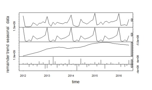
To do a very simple seasonal analysis, we can use the “forecast” package. The stl command allows us to see an underlying trend, a seasonal adjustment, and a residual error. I’ll plot just my time series data with seasonal model (fit).
install.packages('forecast')
library(forecast)
mts <- ts(revtotal$monthly_revenue,
     start=c(2012,1),end=c(2016,6),frequency=12)
fit <- stl(mts, s.window="period")
plot(fit)
Hope this tutorial has encouraged you to play around with new sources of data.
