Bootstrap is one of the most famous resampling technique and is very useful to get confidence intervals in situations where classical approach (t- or z- tests) would fail.
What is bootstrap
Instead of writing down some equations let’s directly see how one may perform bootstrap. Below we will show a simple bootstrap example using the height of 100 person in the population.
set.seed(20151101)
height<-rnorm(100,175,6)
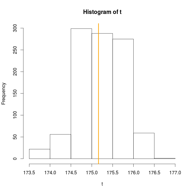
Now we will resample with replacement 1000 times and compute the median:
t0<-median(height)
t<-sapply(1:1000,function(x) median(sample(x=height,size=100,replace=TRUE)))
hist(t)
abline(v=t0,col="orange",lwd=3)
And that’s it, this is the essence of bootstrap: resampling the observed data with replacement and computing the statistic of interest (here the median) many times on the resampled data to get a distribution of the statistic of interest. This distribution of the statistic of interest can then be used to compute, for example, confidence intervals.
When to use bootstrap
Bootstrap is used to enable inference on the statistic of interest when the true distribution of this statistic is unknown. For example in linear model the parameter of interest have a known distribution from which standard errors and formal tests can be performed. On the other hand for some statistics (median, differences between two models …), if the analyst do not want to spend time writing down equations, bootstrapping might be a great approach to get standard errors and confidence intervals from the bootstrapped distribution.
When will bootstrap fail
There are some situations where bootstrapped will fail: (i) the statistic of interest is at the edge of the parameter space (like minimum or maximum), the bootstraped distribution does not converge (as the number of bootstrap sample increase to infinity) to the true distribution of the statistic. (ii) sample size is small, bootstrapping will not increase the power of statistical tests. If you sample to few data to detect an effect of interest, using bootstrap will not magically solve your problem even worse the bootstrap approach will perform less well than others.
How many bootstrap samples
As much as possible will be the answer. Note that in this post I used low numbers to speed up the computations on my “old” computer.
Non-parametric and parametric bootstrap using the boot library
The boot library in R is very convenient to easily compute confidence intervals from bootstrap samples. Non-parametric bootstrap with boot:
library(boot)
b1<-boot(data=height,statistic=function(x,i) median(x[i]),R=1000)
boot.ci(b1)

BOOTSTRAP CONFIDENCE INTERVAL CALCULATIONS
Based on 1000 bootstrap replicates

CALL :
boot.ci(boot.out = b1)

Intervals :
Level      Normal              Basic
95%   (174.1, 176.2 )   (174.2, 176.4 )

Level     Percentile            BCa
95%   (173.9, 176.1 )   (173.8, 176.1 )
Calculations and Intervals on Original Scale
Parametric bootstrap with boot:
x<-runif(100,-2,2)
y<-rnorm(100,1+2*x,1)
dat<-data.frame(x=x,y=y)
Simple example with a linear model
m<-lm(y~x)
We are interested in getting the confidence intervals for the coefficient of the model:
foo<-function(out){
  m<-lm(y~x,out)
  coef(m)
}
The function rgen generate new response vector from the model:
rgen<-function(dat,mle){
  out<-dat
  out$y<-unlist(simulate(mle))
  return(out)
}
Generate 1000 bootstrap sample
b2<-boot(dat,foo,R=1000,sim="parametric",ran.gen=rgen,mle=m)
Compute the confidence intervals for the two coefficients:
boot.ci(b2,type="perc",index=1)

BOOTSTRAP CONFIDENCE INTERVAL CALCULATIONS
Based on 1000 bootstrap replicates

CALL :
boot.ci(boot.out = b2, type = "perc", index = 1)

Intervals :
Level     Percentile
95%   ( 0.8056,  1.1983 )
Calculations and Intervals on Original Scale
Compute the confidence intervals for the two coefficients:
boot.ci(b2,type="perc",index=2)

BOOTSTRAP CONFIDENCE INTERVAL CALCULATIONS
Based on 1000 bootstrap replicates

CALL :
boot.ci(boot.out = b2, type = "perc", index = 2)

Intervals :
Level     Percentile
95%   ( 1.871,  2.217 )
Calculations and Intervals on Original Scale
In the non-parametric case boot expect two arguments in the function returning the statistic of interest: the first one is the object from which to compute the statistic and the second is a vector of index (i), frequencies (f) or weight (w) defining the bootstrap sample. In our example, boot will generate a series of indices (named i) with replacement and these will be used to subset the original height vector. In the parametric case the function returning the statistic(s) of interest only need one argument: the original dataset. We then need to supply another function (ran.gen) describing how to generate the new data, it needs to return an object of the same form as the original dataset. This random data generating function need two arguments: the first one is the original dataset and the second one contain maximum likelihood estimate for the parameter of interest, basically a model object. The new dataset generated by the ran.gen function will then be passed to the statistic function to compute the bootstrapped value for the statistic of interest. It is then straightforward to get the confidence intervals for the statistic using boot.ci.
Bootstrap applied to mixed-effect models
Mixed-effect models are rather complex and the distributions or numbers of degrees of freedom of various output from them (like parameters …) is not known analytically. Which is why the author of the lme4 package recommend the use of bootstrap to get confidence intervals around the model parameters, the predicted values but also to get p-values from likelihood ratio tests.
A simple random intercept model:
dat<-data.frame(x=runif(100,-2,2),ind=gl(n=10,k=10))
dat$y<-1+2*dat$x+rnorm(10,0,1.2)[dat$ind]+rnorm(100,0,0.5)
m<-lmer(y~x+(1|ind),dat)
Get the bootstrapped confidence intervals for the model parameters:
b_par<-bootMer(x=m,FUN=fixef,nsim=200)
boot.ci(b_par,type="perc",index=1)

BOOTSTRAP CONFIDENCE INTERVAL CALCULATIONS
Based on 200 bootstrap replicates

CALL :
boot.ci(boot.out = b_par, type = "perc", index = 1)

Intervals :
Level     Percentile
95%   ( 0.393,  1.824 )
Calculations and Intervals on Original Scale
Some percentile intervals may be unstable
Get the bootstrapped confidence intervals for the model parameters:
boot.ci(b_par,type="perc",index=2)

BOOTSTRAP CONFIDENCE INTERVAL CALCULATIONS
Based on 200 bootstrap replicates

CALL :
boot.ci(boot.out = b_par, type = "perc", index = 2)

Intervals :
Level     Percentile
95%   ( 1.857,  2.041 )
Calculations and Intervals on Original Scale
Some percentile intervals may be unstable
Or alternatively:
confint(m,parm=c(3,4),method="boot",nsim=200,boot.type="perc")

                2.5 %   97.5 %
(Intercept) 0.4337793 1.819856
x           1.8611089 2.058930
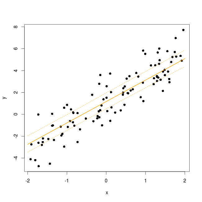
Get the bootstrapped confidence intervals around the regression curves:
new_dat<-data.frame(x=seq(-2,2,length=20))
mm<-model.matrix(~x,data=new_dat)
predFun<-function(.) mm%*%fixef(.)
bb<-bootMer(m,FUN=predFun,nsim=200) #do this 200 times
As we did this 200 times the 95% CI will be bordered by the 5th and 195th value:
bb_se<-apply(bb$t,2,function(x) x[order(x)][c(5,195)])
new_dat$LC<-bb_se[1,]
new_dat$UC<-bb_se[2,]
new_dat$pred<-predict(m,newdata=new_dat,re.form=~0)
Plot the results
plot(y~x,dat,pch=16)
lines(pred~x,new_dat,lwd=2,col="orange")
lines(LC~x,new_dat,lty=2,col="orange")
lines(UC~x,new_dat,lty=2,col="orange")
Finally get bootstrapped p-values from the likelihood ratio test between two models.
library(pbkrtest)
m_0<-update(m,.~.-x)
PBmodcomp(m,m_0,nsim=200)

Parametric bootstrap test; time: 14.35 sec; samples: 200 extremes: 0;
large : y ~ x + (1 | ind)
small : y ~ (1 | ind)
       stat df   p.value
LRT    275.19  1 < 2.2e-16 ***
PBtest 275.19     0.004975 **
---
Signif. codes:  0 '***' 0.001 '**' 0.01 '*' 0.05 '.' 0.1 ' ' 1
Drawing confidence intervals around the regression curves is tricky due to the random effect estimated values which comes with there own uncertainty (have a look at dotplot(ranef(m,condVar=TRUE)) to see it). Bootstrapping is an efficient way to take these uncertainties into account since the random deviates are re-computed for each draw. Finally getting p-values for the effect of a fixed-effect term can be done using a parametric bootstrap approach as described here and implemented in the function PBmodcomp from the pbkrtest package. In the output of PBmodcomp the bootstrapped p-values is in the PBtest line, the LRT line report the standard p-value assuming a chi-square distribution for the LRT value.
Conclusion
With computers being always faster, bootstrap enable us to get reliable confidence interval estimate (given that your original sample size is large enough) without relying on some hypothetical distributions. Bootstrap can also be extended in a bayesian framework, see for example this nice post.
If you have any comments or suggestion feel free to post a comment below.

