The premise of Bayesian statistics is that distributions are based on a personal belief about the shape of such a distribution, rather than the classical assumption which does not take such subjectivity into account.
In this regard, Bayesian statistics defines distributions in the following way:
- Prior: Beliefs about a distribution prior to observing any data.
- Likelihood: Distribution based on the observed data.
- Posterior: Distribution that combines observed data with prior beliefs.
Classical statistics relies largely on the t-test to determine significance of a particular variable, and does not take subjective predictions of the data into account. However, the issue with such an approach is that no constraint is placed on the data, and as Richard Morey explains in his blog, an alternative hypothesis becomes “completely unfalsifiable”.
In this regard, the Bayes factor penalizes hypotheses that are not specific enough, allowing for a more concrete assessment of how accurate a specific prediction is.
Problem and hypothesis
As an example, let us consider the hypothesis that BMI increases with age. Conversely, the null hypothesis argues that there is no evidence for a positive correlation between BMI and age.
In this regard, even if we did find a positive correlation between BMI and age, the hypothesis is virtually unfalsifiable given that the existence of no relationship whatever between these two variables is highly unlikely.
Therefore, as opposed to using a simple t-test, a Bayes Factor analysis needs to have specific predictions to assess the accuracy of the same.
t-test vs. Bayes Factor t-test
For this problem, the diabetes dataset from the UCI Machine Learning Repository is used. The variables Age and BMI are extracted, the data is ordered by age, and a t-test is calculated across two separate age groups.
library(BayesFactor)

# Data Processing
health<-read.csv("diabetes.csv")
attach(health)
newdata <- data.frame(Age,BMI)
newdata <- newdata[order(Age),]

## Compute difference scores
diffScores = newdata$BMI[1:384] - newdata$BMI[385:768]

## Traditional two-tailed t test
t.test(diffScores)
data:  diffScores
t = -2.2622, df = 383, p-value = 0.02425
alternative hypothesis: true mean is not equal to 0
95 percent confidence interval:
 -2.4371984 -0.1706141
sample estimates:
mean of x
-1.303906
With a p-value below 0.05, the t-test shows significance at the 5% level, indicating that the null hypothesis of the mean is equal to 0 is rejected. However, the issue still remains in that the degree of evidence in favor of H1 over H0 cannot be quantified in detail.
In this regard, a Bayes Factor t-test is run across the different scores.
bf = ttestBF(x = diffScores)
bf
Bayes factor analysis
--------------
[1] Alt., r=0.707 : 0.7139178 ±0.01%

Against denominator:
  Null, mu = 0
---
Bayes factor type: BFoneSample, JZS
A score of 0.7139 is yielded. Typically, a score of > 1 signifies anecdotal evidence for H0 compared to H1. The exact thresholds are defined by Wagenmakers et. al, 2011, and a copy of the table can be found at the following The 20% Statistician post.
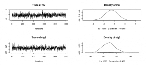
Let’s come back to the issue of the posterior distribution. In the case that we are unable to calculate the posterior distribution, it can be estimated using Markov chain Monte Carlo methods (MCMC).
The chains are estimated and the distributions are plotted:
chains = posterior(bf, iterations = 1000)
summary(chains)
plot(chains[,1:2])
Iterations = 1:1000
Thinning interval = 1
Number of chains = 1
Sample size per chain = 1000

1. Empirical mean and standard deviation for each variable,
   plus standard error of the mean:

          Mean       SD Naive SE Time-series SE
mu     -1.2667  0.56619 0.017904       0.017904
sig2  128.3996  9.42371 0.298004       0.298004
delta  -0.1121  0.05032 0.001591       0.001591
g       1.8037 10.59165 0.334937       0.334937

2. Quantiles for each variable:

           2.5%      25%      50%       75%     97.5%
mu     -2.38323  -1.6611  -1.2626  -0.87649  -0.17530
sig2  111.81072 121.7486 128.2914 134.16920 147.16271
delta  -0.21117  -0.1458  -0.1123  -0.07679  -0.01459
g       0.06183   0.1763   0.3868   0.94495   8.79583
Here is the graph of the distributions:

regressionBF
Bayesian analysis can also be used to compare probabilities across several regression models.
As an example, let’s take the following regression model:
reg1 = lm(BMI ~ Insulin + Age + BloodPressure + Glucose + Pregnancies, data = health)
summary(reg1)
Call:
lm(formula = BMI ~ Insulin + Age + BloodPressure + Glucose +
    Pregnancies, data = health)

Residuals:
    Min      1Q  Median      3Q     Max
-33.502  -4.559  -0.220   4.400  29.738

Coefficients:
               Estimate Std. Error t value Pr(>|t|)
(Intercept)   20.669900   1.375338  15.029  < 2e-16 ***
Insulin        0.008192   0.002486   3.295  0.00103 **
Age           -0.044086   0.028317  -1.557  0.11992
BloodPressure  0.106763   0.014281   7.476 2.11e-13 ***
Glucose        0.038988   0.009258   4.211 2.84e-05 ***
Pregnancies    0.011194   0.094427   0.119  0.90567
---
Signif. codes:  0 ‘***’ 0.001 ‘**’ 0.01 ‘*’ 0.05 ‘.’ 0.1 ‘ ’ 1

Residual standard error: 7.377 on 762 degrees of freedom
Multiple R-squared:  0.1302,	Adjusted R-squared:  0.1245
F-statistic: 22.81 on 5 and 762 DF,  p-value: < 2.2e-16
Again, we see that certain variables are indicated as statistically significant while others are not. However, the same problem arises in that p-values are not regarded as direct measures of evidence against the null hypothesis under the Bayesian school of thought, and thus more concrete probability measures should be used.
In this regard, a Bayesian regression is run, with a Bayes factor analysis indicating the highest and lowest probability regressions.
bf = regressionBF(BMI ~ Insulin + Age + BloodPressure + Glucose + Pregnancies, data = health)
length(bf)
[1] 31
head(bf, 3)
Bayes factor analysis
--------------
[1] Insulin + BloodPressure + Glucose               : 1.352293e+19 ±0%
[2] Insulin + Age + BloodPressure + Glucose         : 7.763347e+18 ±0%
[3] Insulin + BloodPressure + Glucose + Pregnancies : 2.389623e+18 ±0.01%

Against denominator:
  Intercept only
---
Bayes factor type: BFlinearModel, JZS
tail(bf, 3)
Bayes factor analysis
--------------
[1] Age               : 0.1321221  ±0%
[2] Pregnancies       : 0.09066687 ±0%
[3] Age + Pregnancies : 0.01652438 ±0.01%

Against denominator:
  Intercept only
---
Bayes factor type: BFlinearModel, JZS
which.max(bf)
Insulin + BloodPressure + Glucose
                               19
From here, we see that the following three combinations of variables in each regression demonstrate the reported highest probability in computing BMI:
- Insulin + BloodPressure + Glucose
- Insulin + Age + BloodPressure + Glucose
- Insulin + BloodPressure + Glucose + Pregnancies
Conversely, these three combinations of variables demonstrated the lowest reported probability:
- Age
- Pregnancies
- Age + Pregnancies
As indicated by which.max(bf), 19 regression models were generated in total.
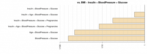
In order to generate a plot of the probabilities for each combination, the probabilities of the top reported models can be divided against the probabilities of all the generated models:
bf2 = head(bf) / max(bf)
bf2
Bayes factor analysis
--------------
[1] Insulin + BloodPressure + Glucose                     : 1          ±0%
[2] Insulin + Age + BloodPressure + Glucose               : 0.5740878  ±0%
[3] Insulin + BloodPressure + Glucose + Pregnancies       : 0.176709   ±0.01%
[4] Insulin + Age + BloodPressure + Glucose + Pregnancies : 0.08419853 ±0%
[5] Age + BloodPressure + Glucose                         : 0.02216035 ±0%
[6] BloodPressure + Glucose                               : 0.01570813 ±0.01%

Against denominator:
  BMI ~ Insulin + BloodPressure + Glucose
---
Bayes factor type: BFlinearModel, JZS
plot(bf2)
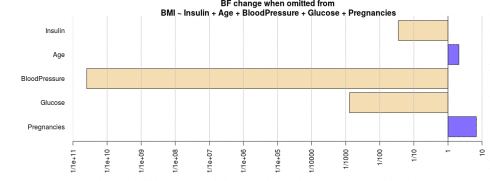
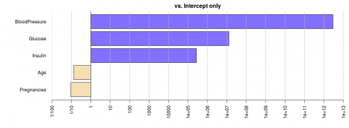
Additionally, “top-down” and “bottom-up” analyses can be generated, wherein the former each independent variable is eliminated one at a time, whereas in the latter each independent variable is added one at a time.
bf_top
Bayes factor top-down analysis
--------------
When effect is omitted from Insulin + Age + BloodPressure + Glucose + Pregnancies , BF is...
[1] Omit Pregnancies   : 6.818265     ±0%
[2] Omit Glucose       : 0.001291526  ±0%
[3] Omit BloodPressure : 2.526265e-11 ±0%
[4] Omit Age           : 2.098719     ±0.01%
[5] Omit Insulin       : 0.0350438    ±0%

Against denominator:
  BMI ~ Insulin + Age + BloodPressure + Glucose + Pregnancies
---
Bayes factor type: BFlinearModel, JZS
plot(bf_top)
# Bottom-up
bf_btm = regressionBF(BMI ~ Insulin + Age + BloodPressure + Glucose + Pregnancies, data = health, whichModels = "bottom")
bf_btm
|=================================================================| 100%
Bayes factor analysis
--------------
[1] Insulin       : 275178       ±0%
[2] Age           : 0.1321221    ±0%
[3] BloodPressure : 2.926062e+12 ±0%
[4] Glucose       : 12805251     ±0%
[5] Pregnancies   : 0.09066687   ±0%

Against denominator:
  Intercept only
---
Bayes factor type: BFlinearModel, JZS
plot(bf_btm)
According to these two graphs, Blood Pressure is indicated as the most influential variable in explaining the indicative probability favoring H1 over H0.
Conclusion
Ultimately, the area of Bayesian statistics is very large and the examples above cover just the tip of the iceberg.
However, in this particular example we have looked at:
- The comparison between a t-test and the Bayes Factor t-test
- How to estimate posterior distributions using Markov chain Monte Carlo methods (MCMC)
- Use of regressionBF to compare probabilities across regression models
Many thanks for your time.


