In a previous post we saw how to perform bayesian regression in R using STAN for normally distributed data. In this post we will look at how to fit non-normal model in STAN using three example distributions commonly found in empirical data: negative-binomial (overdispersed poisson data), gamma (right-skewed continuous data) and beta-binomial (overdispersed binomial data).
The STAN code for the different models is at the end of this posts together with some explanations.
Negative Binomial
The Poisson distribution is a common choice to model count data, it assumes that the variance is equal to the mean. When the variance is larger than the mean, the data are said to be overdispersed and the Negative Binomial distribution can be used. Say we have measured a response variable y that follow a negative binomial distribution and depends on a set of k explanatory variables X, in equation this gives us:
$$ y_{i} \sim NB(\mu_{i},\phi) $$ $$ E(y_{i}) = \mu_{i} $$ $$ Var(y_{i}) = \mu_{i} + \mu_{i}^{2} / \phi $$ $$ log(\mu_{i}) = \beta_{0} + \beta_{1} * X1_{i} + … + \beta_{k} * Xk_{i} $$
The negative binomial distribution has two parameters: \(\mu\) is the expected value that need to be positive, therefore a log link function can be used to map the linear predictor (the explanatory variables times the regression parameters) to \(\mu\) (see the 4th equation); and \(\phi\) is the overdispersion parameter, a small value means a large deviation from a Poisson distribution, while as \(\phi\) gets larger the negative binomial looks more and more like a Poisson distribution.
Let’s simulate some data and fit a STAN model to them:
#load the libraries
library(arm) #for the invlogit function
library(emdbook) #for the rbetabinom function
library(rstan)
library(rstanarm) #for the launch_shinystan function

#simulate some negative binomial data
#the explanatory variables
N<-100 #sample size
dat<-data.frame(x1=runif(N,-2,2),x2=runif(N,-2,2))
#the model
X<-model.matrix(~x1*x2,dat)
K<-dim(X)[2] #number of regression params
#the regression slopes
betas<-runif(K,-1,1)
#the overdispersion for the simulated data
phi<-5
#simulate the response
y_nb<-rnbinom(100,size=phi,mu=exp(X%*%betas))

#fit the model
m_nb<-stan(file = "neg_bin.stan",data = list(N=N,K=K,X=X,y=y_nb),pars=c("beta","phi","y_rep"))

#diagnose and explore the model using shinystan
launch_shinystan(m_nb)
The last command should open a window in your browser with loads of options to diagnose, estimate and explore your model. Some options are beyond my limited knowledge (ie Log Posterior vs Sample Step Size), so I usually look at the posterior distribution of the regression parameters (Diagnose -> NUTS (plots) -> By model parameter), the histogram should be more or less normal. I also look at Posterior Predictive Checks (Diagnose -> PPcheck -> Distribution of observed data vs replications), the distribution of the y_rep should be equivalent to the observed data.
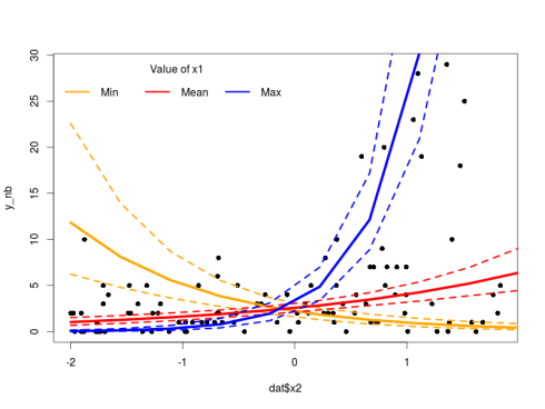
The model looks fine, we can now plot the predicted regression lines with their credible intervals using the sampled regression parameters from the model:
#get the posterior predicted values together with the credible intervals
post<-as.array(m_nb) #the sampled model values
#will look at varying x2 with 3 values of x1
new_X<-model.matrix(~x1*x2,expand.grid(x2=seq(-2,2,length=10),x1=c(min(dat$x1),mean(dat$x1),max(dat$x1))))
#get the predicted values for each samples
pred<-apply(post[,,1:4],c(1,2),FUN = function(x) new_X%*%x)
#each chains is in a different matrix re-group the info into one matrix
dim(pred)<-c(30,4000)
#get the median prediction plus 95% credible intervals
pred_int<-apply(pred,1,quantile,probs=c(0.025,0.5,0.975))

#plot
plot(dat$x2,y_nb,pch=16)
lines(new_X[1:10,3],exp(pred_int[2,1:10]),col="orange",lwd=5)
lines(new_X[1:10,3],exp(pred_int[1,1:10]),col="orange",lwd=3,lty=2)
lines(new_X[1:10,3],exp(pred_int[3,1:10]),col="orange",lwd=3,lty=2)
lines(new_X[1:10,3],exp(pred_int[2,11:20]),col="red",lwd=5)
lines(new_X[1:10,3],exp(pred_int[1,11:20]),col="red",lwd=3,lty=2)
lines(new_X[1:10,3],exp(pred_int[3,11:20]),col="red",lwd=3,lty=2)
lines(new_X[1:10,3],exp(pred_int[2,21:30]),col="blue",lwd=5)
lines(new_X[1:10,3],exp(pred_int[1,21:30]),col="blue",lwd=3,lty=2)
lines(new_X[1:10,3],exp(pred_int[3,21:30]),col="blue",lwd=3,lty=2)
legend("topleft",legend=c("Min","Mean","Max"),ncol=3,col = c("orange","red","blue"),lwd = 3,bty="n",title="Value of x1")
As always with such models one must pay attention to the difference between the link and the response space. The model makes prediction in the link space, if we want to plot them next to the actual response value we need to apply the inverse of the link function (in our case exponentiate the values) to back-transform the model prediction.
Gamma distribution
Sometime we collect continuous data that show right-skew, like body sizes or plant biomass, such data may be modelled using a log-normal distribution (basically log-transforming the reponse) or using a gamma distribution (see this discussion). Here I will look at gamma distribution, say we collected some gamma-distributed y responding to some explanatory variable X, in equation this gives us:
$$ y_{i} \sim Gamma(\alpha,\beta) $$ $$ E(y_{i}) = \alpha / \beta $$ $$ Var(y_{i}) = \alpha / \beta^{2} $$
Mmmmmmm in contrary to the negative binomial above we cannot directly map the linear predictor directly to one parameter of the model (\(\mu\) for example). So we need to re-parametrize the model by doing some calculus:
$$ E(y_{i}) = \alpha / \beta = \mu $$ $$ Var(y_{i}) = \alpha / \beta^{2} = \phi $$
Re-arranging gives us:
$$ \alpha = \mu^{2} / \phi $$ $$ \beta = \mu / \phi $$
Where \(\mu\) is now our expected value and \(\phi\) a dispersion parameter like in the Negative Binomial example above. As \(\alpha\) and \(\beta\) must be positive we can use again a log link on the linear predictor:
$$ log(\mu_{i}) = \beta_{0} + \beta_{1} * X1_{i} + … + \beta_{k} * Xk_{i} $$
Let’s simulate some data and fit a model to this:
#simulate gamma data
mus<-exp(X%*%betas)
y_g<-rgamma(100,shape=mus**2/phi,rate=mus/phi)

#model
m_g<-stan(file = "gamma.stan",data = list(N=N,K=K,X=X,y=y_g),pars=c("betas","phi","y_rep"))

#model check
launch_shinystan(m_g)
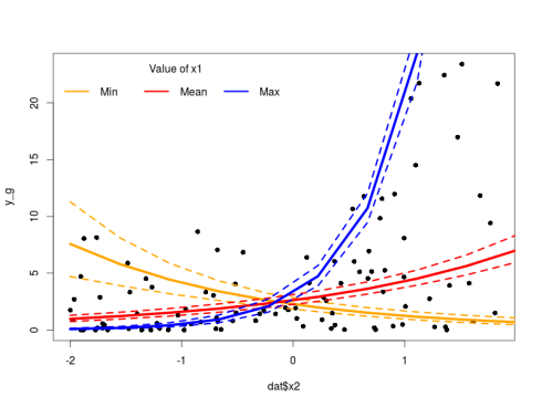
Again we check that the model is correct, everything is very nice on this front. We can plot the results using similar code as above replacing m_nb by m_g. Since we used the same link function in the Negative Binomial and the Gamma model the rest will work.
Beta-binomial
Finally when we collect data from a certain number of trials (I throw ten time a coin what is the proportion of heads?) the response usually follows a binomial distribution. Now empirical data are messy and just like Poisson data may be overdispersed, so can binomial be. To account for this the Beta-Binomial model can be used:
$$ y_{i} \sim BetaBinomial(N,\alpha,\beta) $$ $$ E(y_{i}) = N*\alpha / (\alpha + \beta) $$
Leaving the variance expression aside (have a look here to see how ugly it is), and the constant N (the number of trials), we can like in the Gamma example re-parametrize the equations to an expected value of \(\mu\) and a dispersion parameter \(\phi\):
$$ \alpha = \mu * \phi $$ $$ \beta = (1-\mu) * \phi $$
This time the \(\mu\) represent a probability and must therefore be between 0 and 1, one can use the logit link to map the linear predictor to \(\mu\):
$$ logit(\mu) = \beta_{0} + \beta_{1} * X1_{i} + … + \beta_{k} * Xk_{i} $$
Again simulation power:
#simulate beta-binomial data
W<-rep(20,100) #number of trials
y_bb<-rbetabinom(100,prob=invlogit(X%*%betas),size=W,theta=phi)

#model
m_bb<-stan(file = "beta_bin.stan",data = list(N=N,W=W,K=K,X=X,y=y_bb),pars=c("betas","phi","y_rep"))

#model check
launch_shinystan(m_bb)
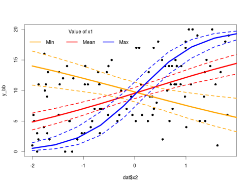
Everything is great, we can now plot this:
#get the posterior predicted values together with the credible intervals
post<-as.array(m_bb) #the posterior draw
#get the predicted values
pred<-apply(post[,,1:4],c(1,2),FUN = function(x) new_X%*%x)
#each chains is in a different matrix re-group the info
dim(pred)<-c(30,4000)
#get the median prediction plus 95% credible intervals
pred_int<-apply(pred,1,quantile,probs=c(0.025,0.5,0.975))

#plot
plot(dat$x2,y_bb,pch=16)
lines(new_X[1:10,3],20*invlogit(pred_int[2,1:10]),col="orange",lwd=5)
lines(new_X[1:10,3],20*invlogit(pred_int[1,1:10]),col="orange",lwd=3,lty=2)
lines(new_X[1:10,3],20*invlogit(pred_int[3,1:10]),col="orange",lwd=3,lty=2)
lines(new_X[1:10,3],20*invlogit(pred_int[2,11:20]),col="red",lwd=5)
lines(new_X[1:10,3],20*invlogit(pred_int[1,11:20]),col="red",lwd=3,lty=2)
lines(new_X[1:10,3],20*invlogit(pred_int[3,11:20]),col="red",lwd=3,lty=2)
lines(new_X[1:10,3],20*invlogit(pred_int[2,21:30]),col="blue",lwd=5)
lines(new_X[1:10,3],20*invlogit(pred_int[1,21:30]),col="blue",lwd=3,lty=2)
lines(new_X[1:10,3],20*invlogit(pred_int[3,21:30]),col="blue",lwd=3,lty=2)
legend("topleft",legend=c("Min","Mean","Max"),ncol=3,col = c("orange","red","blue"),lwd = 3,bty="n",title="Value of x1")
Note the change from exp to invlogit taking into account the different link function used.
Parting thoughts
In this post we saw how to adapt our models to non-normal data that are pretty common out there. STAN is very flexible and allow many different parametrization for many different distributions (see the reference guide), the possibilities are only limited by your hypothesis (and maybe a bit your mathematical skills …). At this point I’d like you to note that the rstanarm package allows you to fit STAN model without you having to write down the model. Instead using the typical R syntax one would use in, for example, a glm call (see this post). So why bothering learning all this STAN stuff? It depends: if you are only fitting “classical” models to your data with little fanciness then just use rstanarm this will save you some time to do your science and the models in this package are certainly better parametrized (ie faster) than the one I presented here. On the other hand if you feel that one day you will have to fit your own customized models then learning STAN is a good way to tap into a highly flexible and powerful language that will keep growing.
Model Code
Negative Binomial:
/*
*Simple negative binomial regression example
*using the 2nd parametrization of the negative
*binomial distribution, see section 40.1-3 in the Stan
*reference guide
*/

data {
  int N; //the number of observations
  int K; //the number of columns in the model matrix
  int y[N]; //the response
  matrix[N,K] X; //the model matrix
}
parameters {
  vector[K] beta; //the regression parameters
  real phi; //the overdispersion parameters
}
transformed parameters {
  vector[N] mu;//the linear predictor
  mu <- exp(X*beta); //using the log link
}
model {
  beta[1] ~ cauchy(0,10); //prior for the intercept following Gelman 2008

  for(i in 2:K)
   beta[i] ~ cauchy(0,2.5);//prior for the slopes following Gelman 2008

  y ~ neg_binomial_2(mu,phi);
}
generated quantities {
 vector[N] y_rep;
 for(n in 1:N){
  y_rep[n] <- neg_binomial_2_rng(mu[n],phi); //posterior draws to get posterior predictive checks
 }
}
Gamma:
/*
*Simple gamma example
*Note that I used a log link which makes
*more sense in most applied cases
*than the canonical inverse link
*/

data {
  int N; //the number of observations
  int K; //the number of columns in the model matrix
  real y[N]; //the response
  matrix[N,K] X; //the model matrix
}
parameters {
  vector[K] betas; //the regression parameters
  real phi; //the variance parameter
}
transformed parameters {
  vector[N] mu; //the expected values (linear predictor)
  vector[N] alpha; //shape parameter for the gamma distribution
  vector[N] beta; //rate parameter for the gamma distribution

  mu <- exp(X*betas); //using the log link
  alpha <- mu .* mu / phi;
  beta <- mu / phi;
}
model {
  betas[1] ~ cauchy(0,10); //prior for the intercept following Gelman 2008

  for(i in 2:K)
   betas[i] ~ cauchy(0,2.5);//prior for the slopes following Gelman 2008

  y ~ gamma(alpha,beta);
}
generated quantities {
 vector[N] y_rep;
 for(n in 1:N){
  y_rep[n] <- gamma_rng(alpha[n],beta[n]); //posterior draws to get posterior predictive checks
 }
}
Beta-Binomial:
/*
*Simple beta-binomial example
*/

data {
  int N; //the number of observations
  int K; //the number of columns in the model matrix
  int y[N]; //the response
  matrix[N,K] X; //the model matrix
  int W[N]; //the number of trials per observations, ie a vector of 1 for a 0/1 dataset
}
parameters {
  vector[K] betas; //the regression parameters
  real phi; //the overdispersion parameter
}
transformed parameters {
  vector[N] mu; //the linear predictor
  vector[N] alpha; //the first shape parameter for the beta distribution
  vector[N] beta; //the second shape parameter for the beta distribution

  for(n in 1:N)
   mu[n] <- inv_logit(X[n,]*betas); //using logit link
  alpha <- mu * phi;
  beta <- (1-mu) * phi;
}
model {
  betas[1] ~ cauchy(0,10); //prior for the intercept following Gelman 2008

  for(i in 2:K)
   betas[i] ~ cauchy(0,2.5);//prior for the slopes following Gelman 2008

  y ~ beta_binomial(W,alpha,beta);
}
generated quantities {
 vector[N] y_rep;
 for(n in 1:N){
  y_rep[n] <- beta_binomial_rng(W[n],alpha[n],beta[n]); //posterior draws to get posterior predictive checks
 }
}
This bring us to the end of the post, if you have any question leave a comment below.


