City of Los Angeles or “The Birthplace of Jazz” is one of the most populous city in the United States of America with the population estimated over four million. With the city of this size, it is worth the effort to explore the crime rate in this city.
The current project is aimed to explore the crime rate in the year 2017. The dataset used in this project is found in this link which is provided by the Los Angeles Police Department.
Date Preparation
library(data.table) #faster way to read large dataset
library(tidyverse) #load dplyr, tidyr and ggplot
library(ggmap) #use to read map
library(maps) #map tools kits
library(mapdata) #read the map data
library(lubridate) #date manuplation
library(ggrepel) #better label
library(varhandle) #load the function unfactor

crime_la <- as.data.frame(fread("Crime_Data_from_2010_to_Present.csv", na.strings = c("NA")))
glimpse(crime_la)
## Observations: 1,805,537
## Variables: 26
## $ `DR Number`              <int> 1208575, 102005556, 418, 101822289, 4...
## $ `Date Reported`          <chr> "03/14/2013", "01/25/2010", "03/19/20...
## $ `Date Occurred`          <chr> "03/11/2013", "01/22/2010", "03/18/20...
## $ `Time Occurred`          <int> 1800, 2300, 2030, 1800, 2300, 1400, 2...
## $ `Area ID`                <int> 12, 20, 18, 18, 21, 1, 11, 16, 19, 9,...
## $ `Area Name`              <chr> "77th Street", "Olympic", "Southeast"...
## $ `Reporting District`     <int> 1241, 2071, 1823, 1803, 2133, 111, 11...
## $ `Crime Code`             <int> 626, 510, 510, 510, 745, 110, 510, 51...
## $ `Crime Code Description` <chr> "INTIMATE PARTNER - SIMPLE ASSAULT", ...
## $ `MO Codes`               <chr> "0416 0446 1243 2000", "", "", "", "0...
## $ `Victim Age`             <int> 30, NA, 12, NA, 84, 49, NA, NA, NA, 2...
## $ `Victim Sex`             <chr> "F", "", "", "", "M", "F", "", "", ""...
## $ `Victim Descent`         <chr> "W", "", "", "", "W", "W", "", "", ""...
## $ `Premise Code`           <int> 502, 101, 101, 101, 501, 501, 108, 10...
## $ `Premise Description`    <chr> "MULTI-UNIT DWELLING (APARTMENT, DUPL...
## $ `Weapon Used Code`       <int> 400, NA, NA, NA, NA, 400, NA, NA, NA,...
## $ `Weapon Description`     <chr> "STRONG-ARM (HANDS, FIST, FEET OR BOD...
## $ `Status Code`            <chr> "AO", "IC", "IC", "IC", "IC", "AA", "...
## $ `Status Description`     <chr> "Adult Other", "Invest Cont", "Invest...
## $ `Crime Code 1`           <int> 626, 510, 510, 510, 745, 110, 510, 51...
## $ `Crime Code 2`           <int> NA, NA, NA, NA, NA, NA, NA, NA, NA, N...
## $ `Crime Code 3`           <int> NA, NA, NA, NA, NA, NA, NA, NA, NA, N...
## $ `Crime Code 4`           <int> NA, NA, NA, NA, NA, NA, NA, NA, NA, N...
## $ Address                  <chr> "6300    BRYNHURST                   ...
## $ `Cross Street`           <chr> "", "15TH", "", "WALL", "", "", "AVEN...
## $ Location                 <chr> "(33.9829, -118.3338)", "(34.0454, -1...
The data used in this project contains 1.8 million observation and 26 variables. The dataset date range from 2010 up until recent 22/08/2018.
Data cleaning
For the purpose of this study only data from the year 2017 is selected. Before the analysis, a simple data analysis such as convert data into a corrected data type, recode the variable into a readable format and select relevant variables is conducted as shown below:
#select relevant variables
crime_la_selected <- select(crime_la, `Date Occurred`, `Time Occurred`, `Area Name`, `Crime Code Description`, `Victim Age`, `Victim Sex`, `Victim Descent`, `Premise Description`, `Weapon Description`, `Status Description`, Location)

#convert the date into date type
crime_la_selected$`Date Occurred` <- mdy(crime_la_selected$`Date Occurred`)

#Separate latitude and longitude
location <- crime_la_selected$Location %>% # take coord as string
  str_replace_all("[()]", "") %>% # replace parantheses
  str_split_fixed(", ", n=2) %>% # split up based on comma and space after
  as.data.frame %>% # turn this to a data frame
  transmute(lat=V1, long=V2) # rename the variables

#combine the lat and long then remove the location
crime_la_selected <- cbind(crime_la_selected, location)

crime_la_selected <- subset(crime_la_selected, select = -c(Location))

#select only 2017 and 2018
crime_selected_years <- filter(crime_la_selected, `Date Occurred` >= as_date("2017-01-01"), `Date Occurred` <= as_date("2017-12-30"))

#remove these data frames to same memory
rm(crime_la, crime_la_selected, location) #remove these data frames to same memory

#separate date into year, month and day.
crime_selected_years$year <- year(crime_selected_years$`Date Occurred`)
crime_selected_years$month <- month(crime_selected_years$`Date Occurred`)
crime_selected_years$days <- day(crime_selected_years$`Date Occurred`)

#Recode the variable into readable format
crime_selected_years$`Victim Sex` <- recode(crime_selected_years$`Victim Sex`, 'F' = 'Female', 'M' = 'Male', 'X' = 'Unknown')

crime_selected_years$`Victim Descent` <- recode(crime_selected_years$`Victim Descent`, "A" = "Other Asian", "B" = "Black", "C" = "Chinese", "D" = "Cambodian", "F" = "Filipino", "G" = "Guamanian", "H" = "Hispanci/Latin/Mexican", 'I' = "American Indian/Alaskan Native", "J" = "Japanese", "K" = "Korean", "L" = "Laotian", "O" = "Other", "P" = "Pacific Islander", "S" = "Somoan", "U" = "Hawaiian", "V" = "Vietnamese", "W" = "White", "X" = "Unknown", "Z" = "Asian Indian")

#convert the character into factor
character_vars <- lapply(crime_selected_years, class) == "character"
crime_selected_years[, character_vars] <- lapply(crime_selected_years[, character_vars], as.factor)

glimpse(crime_selected_years)
## Observations: 229,902
## Variables: 15
## $ `Date Occurred`          <date> 2017-07-20, 2017-07-21, 2017-04-21, ...
## $ `Time Occurred`          <int> 2000, 1000, 1930, 1700, 745, 1, 730, ...
## $ `Area Name`              <fct> West Valley, West Valley, Rampart, Ra...
## $ `Crime Code Description` <fct> BURGLARY FROM VEHICLE, BURGLARY FROM ...
## $ `Victim Age`             <int> 55, 20, 16, 16, 16, 16, 16, 16, 16, 2...
## $ `Victim Sex`             <fct> Male, Male, , , , , , , , Male, , , ,...
## $ `Victim Descent`         <fct> Other, Other, , , , , , , , Black, , ...
## $ `Premise Description`    <fct> , , STREET, STREET, STREET, STREET, S...
## $ `Weapon Description`     <fct> , , , , , , , , , , , , , , , , , , ,...
## $ `Status Description`     <fct> Invest Cont, Invest Cont, Invest Cont...
## $ lat                      <fct> , , 34.0886, 34.0512, 34.0328, 34.067...
## $ long                     <fct> , , -118.2979, -118.2787, -118.2915, ...
## $ year                     <dbl> 2017, 2017, 2017, 2017, 2017, 2017, 2...
## $ month                    <dbl> 7, 7, 4, 2, 4, 4, 4, 3, 5, 6, 1, 2, 3...
## $ days                     <int> 20, 21, 21, 11, 25, 7, 8, 6, 11, 6, 2...
After the data cleaning process, only 229,902 observations and 15 variables are selected.
Total Crime in 2017
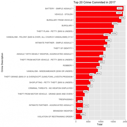
Let’s look at the top 20 of crime that has been committed in 2017.
year_2017 <- crime_selected_years %>%
  filter(year == "2017")

group <- year_2017 %>%
  group_by(`Crime Code Description`) %>%
  summarise(total = n()) %>%
  distinct() %>%
  top_n(20)

group %>%
  ggplot(aes(reorder(`Crime Code Description`, total), y = total)) +
  geom_col(fill = "red") +
  geom_label_repel(aes(label = total), size = 2.5) +
  coord_flip() +
  labs(title = "Top 20 Crime Commited in 2017",
       x = "Crime Description",
       y = "Total")
As you can see, the most crime committed in 2017 are battery-simple assault, stolen vehicle, and burglary from a vehicle.
Age group
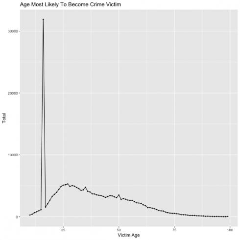
Next I'm going to examine the age group most likely to become victim of crime.
age <- year_2017 %>%
  group_by(`Victim Age`) %>%
  summarise(total = n()) %>%
  na.omit()

age %>%
  ggplot(aes(x = `Victim Age`, y = total)) +
  geom_line(group = 1) +
  geom_point(size = 0.5) +
  labs(title = "Age Most Likely To Become Crime Victim",
       x = "Victim Age",
       y = "Total")
As shown above, the age group below 25 are most likely to become victim of crime in 2017. The huge spike is represented as age 16.
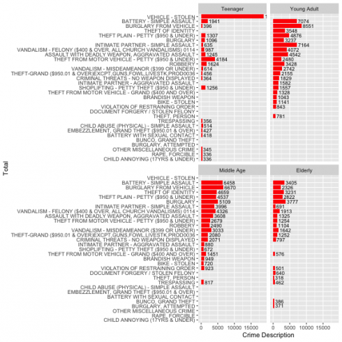
Next I'm going to factor the age into different group and examine which crime are targeted to different age group. I going to cut the age group into teenager (10-18), young adult, (19 – 35), middle age (36-55) and elderly (56 above)
year_2017$age_group <- cut(year_2017$`Victim Age`, breaks = c(-Inf, 19, 35, 55, Inf), labels = c("Teenager", "Young Adult", "Middle Age", "Elderly"))

age.group <- year_2017 %>%
  group_by(age_group, `Crime Code Description`) %>%
  summarise(total = n()) %>%
  top_n(20) %>%
  na.omit()

age.group %>%
  ggplot(aes(reorder(x = `Crime Code Description`, total), y = total)) +
  geom_col(fill = 'red') +
  geom_text(aes(label=total), color='black', hjust = -0.1, size = 3) +
  coord_flip() +
  facet_wrap(~ age_group) +
  labs(x = 'Total',
       y = "Crime Description")
As you can see there are different crime target to different age group.
Gender
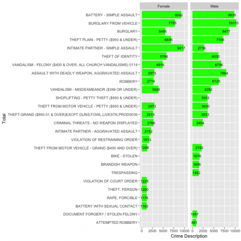
In this section, I'm going to examine type of crime targeted to different gender.
gender <- year_2017 %>%
  group_by(`Victim Sex`, `Crime Code Description`) %>%
  summarise(total = n()) %>%
  filter(`Victim Sex` != "Unknown", `Victim Sex` != "H") %>%
  na.omit() %>%
  top_n(20)

gender <- gender[-c(1:30),]

gender %>%
  ggplot(aes(reorder(x = `Crime Code Description`, total), y = total)) +
  geom_col(fill = 'green') +
  geom_text(aes(label=total), color='black', hjust = 0.8, size = 3) +
  coord_flip() +
  facet_wrap(~ `Victim Sex`) +
  labs(x = 'Total',
       y = "Crime Description")
As you can see both gender are likely to be victim of different kind of crime.
Map The Crime
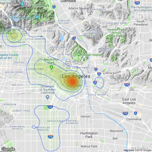
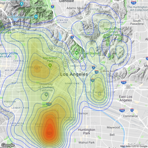
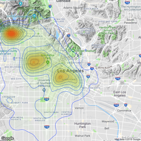
Next we are going to map the crime. For the illustrate purpose, I'm going to map only the the highest crime commited in 2017 which were assualt vehicle stolen and burgarly from vehicle.
#get the map of LA
LA_map <- qmap(location = "Los Angeles", zoom = 12)

#unfactor variable
year_2017$lat <- unfactor(year_2017$lat)
year_2017$long <- unfactor(year_2017$long)

#select relevant variables
mapping <- year_2017 %>%
  select(`Crime Code Description`, long, lat) %>%
  filter(`Crime Code Description` == 'BATTERY - SIMPLE ASSAULT') %>%
  na.omit()

#mapping
LA_map + geom_density_2d(aes(x = long, y = lat), data = mapping) +
  stat_density2d(data = mapping,
    aes(x = long, y = lat, fill = ..level.., alpha = ..level..), size = 0.01,
    bins = 16, geom = "polygon") + scale_fill_gradient(low = "green", high = "red",
    guide = FALSE) + scale_alpha(range = c(0, 0.3), guide = FALSE)
As you can see the battery assault is more likely to happen on Downtown Los Angeles.
mapping <- year_2017 %>%
  select(`Crime Code Description`, long, lat) %>%
  filter(`Crime Code Description` == 'VEHICLE - STOLEN') %>%
  na.omit()

LA_map + geom_density_2d(aes(x = long, y = lat), data = mapping) +
  stat_density2d(data = mapping,
    aes(x = long, y = lat, fill = ..level.., alpha = ..level..), size = 0.01,
    bins = 16, geom = "polygon") + scale_fill_gradient(low = "green", high = "red",
    guide = FALSE) + scale_alpha(range = c(0, 0.3), guide = FALSE)
Interestingly, most vehicle are more likely to be stolen on South Los Angeles.
mapping <- year_2017 %>%
  select(`Crime Code Description`, long, lat) %>%
  filter(`Crime Code Description` == 'BURGLARY FROM VEHICLE') %>%
  na.omit()

LA_map + geom_density_2d(aes(x = long, y = lat), data = mapping) +
  stat_density2d(data = mapping,
    aes(x = long, y = lat, fill = ..level.., alpha = ..level..), size = 0.01,
    bins = 16, geom = "polygon") + scale_fill_gradient(low = "green", high = "red",
    guide = FALSE) + scale_alpha(range = c(0, 0.3), guide = FALSE)
The heatmap shows that Hollywood, Koreatown and Downtown Los Angeles have the highest chance of getting burgalry from vehicle.
Conclusion
This is just a simple demonstration of how to gain insight of the data and mapping the crime in Los Angeles.
