Market Basket Analysis is one of the key techniques used by large retailers to uncover associations between items. It works by looking for combinations of items that occur together frequently in transactions. To put it another way, it allows retailers to identify relationships between the items that people buy.
Association Rules are widely used to analyze retail basket or transaction data, and are intended to identify strong rules discovered in transaction data using measures of interestingness, based on the concept of strong rules.
An example of Association Rules
-
* Assume there are 100 customers
* 10 of them bought milk, 8 bought butter and 6 bought both of them
* bought milk => bought butter
* support = P(Milk & Butter) = 6/100 = 0.06
* confidence = support/P(Butter) = 0.06/0.08 = 0.75
* lift = confidence/P(Milk) = 0.75/0.10 = 7.5
Note: this example is extremely small. In practice, a rule needs the support of several hundred transactions, before it can be considered statistically significant, and datasets often contain thousands or millions of transactions.
Ok, enough for the theory, let’s get to the code.
The dataset we are using today comes from UCI Machine Learning repository. The dataset is called “Online Retail” and can be found here. It contains all the transactions occurring between 01/12/2010 and 09/12/2011 for a UK-based and registered online retailer.
Load the packages
library(tidyverse)
library(readxl)
library(knitr)
library(ggplot2)
library(lubridate)
library(arules)
library(arulesViz)
library(plyr)
Data preprocessing and exploring
retail <- read_excel('Online_retail.xlsx')
retail <- retail[complete.cases(retail), ]
retail %>% mutate(Description = as.factor(Description))
retail %>% mutate(Country = as.factor(Country))
retail$Date <- as.Date(retail$InvoiceDate)
retail$Time <- format(retail$InvoiceDate,"%H:%M:%S")
retail$InvoiceNo <- as.numeric(as.character(retail$InvoiceNo))
glimpse(retail)
Observations: 406,829
Variables: 10
$ InvoiceNo    536365, 536365, 536365, 536365, 536365, 536365, 536365, 53...
$ StockCode    "85123A", "71053", "84406B", "84029G", "84029E", "22752", ...
$ Description  WHITE HANGING HEART T-LIGHT HOLDER, WHITE METAL LANTERN, ...
$ Quantity     6, 6, 8, 6, 6, 2, 6, 6, 6, 32, 6, 6, 8, 6, 6, 3, 2, 3, 3, ...
$ InvoiceDate  2010-12-01 08:26:00, 2010-12-01 08:26:00, 2010-12-01 08:2...
$ UnitPrice    2.55, 3.39, 2.75, 3.39, 3.39, 7.65, 4.25, 1.85, 1.85, 1.69...
$ CustomerID   17850, 17850, 17850, 17850, 17850, 17850, 17850, 17850, 17...
$ Country      United Kingdom, United Kingdom, United Kingdom, United Ki...
$ Date         2010-12-01, 2010-12-01, 2010-12-01, 2010-12-01, 2010-12-0...
$ Time         "08:26:00", "08:26:00", "08:26:00", "08:26:00", "08:26:00"...
After preprocessing, the dataset includes 406,829 records and 10 fields: InvoiceNo, StockCode, Description, Quantity, InvoiceDate, UnitPrice, CustomerID, Country, Date, Time.
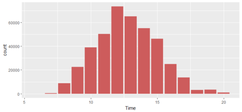
What time do people often purchase online?
In order to find the answer to this question, we need to extract “hour” from the time column.
retail$Time <- as.factor(retail$Time)
a %>%
  ggplot(aes(x=Time)) +
  geom_histogram(stat="count",fill="indianred")
There is a clear bias between the hour of day and order volume. Most orders happened between 10:00–15:00.
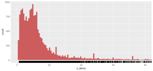
How many items each customer buy?
detach("package:plyr", unload=TRUE)
retail %>%
  group_by(InvoiceNo) %>%
  summarize(n_items = mean(Quantity)) %>%
  ggplot(aes(x=n_items))+
  geom_histogram(fill="indianred", bins = 100000) +
  geom_rug()+
  coord_cartesian(xlim=c(0,80))
People mostly purchased less than 10 items (less than 10 items in each invoice).
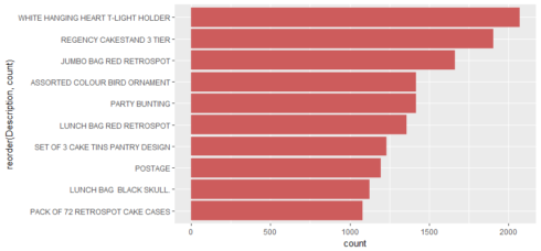
Top 10 best sellers
tmp %>%
  group_by(StockCode, Description) %>%
  summarize(count = n()) %>%
  arrange(desc(count))
tmp %>%
  ggplot(aes(x=reorder(Description,count), y=count))+
  geom_bar(stat="identity",fill="indian red")+
  coord_flip()
# A tibble: 10 x 3
# Groups:   StockCode [10]
   StockCode                        Description count

 1    85123A WHITE HANGING HEART T-LIGHT HOLDER  2070
 2     22423           REGENCY CAKESTAND 3 TIER  1905
 3    85099B            JUMBO BAG RED RETROSPOT  1662
 4     84879      ASSORTED COLOUR BIRD ORNAMENT  1418
 5     47566                      PARTY BUNTING  1416
 6     20725            LUNCH BAG RED RETROSPOT  1358
 7     22720   SET OF 3 CAKE TINS PANTRY DESIGN  1232
 8      POST                            POSTAGE  1196
 9     20727            LUNCH BAG  BLACK SKULL.  1126
10     21212    PACK OF 72 RETROSPOT CAKE CASES  1080
Association rules for online retailer
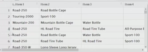
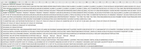
Before using any rule mining algorithm, we need to transform the data from the data frame format, into transactions such that we have all the items bought together in one row. For example, this is the format we need:
retail_sorted <- retail[order(retail$CustomerID),]
library(plyr)
itemList <- ddply(retail,c("CustomerID","Date"),
                       function(df1)paste(df1$Description,
                       collapse = ","))
The function ddply() accepts a data frame, splits it into pieces based on one or more factors, computes on the pieces, and then returns the results as a data frame. We use “,” to separate different items.
We only need item transactions, so remove customerID and Date columns.
itemList$CustomerID <- NULL
itemList$Date <- NULL
colnames(itemList) <- c("items")
Write the data fram to a csv file and check whether our transaction format is correct.
write.csv(itemList,"market_basket.csv", quote = FALSE, row.names = TRUE)
Perfect! Now we have our transaction dataset, and it shows the matrix of items being bought together. We don’t actually see how often they are bought together, and we don’t see rules either. But we are going to find out.
Let’s have a closer look at how many transactions we have and what they are.
tr <- read.transactions('market_basket.csv', format = 'basket', sep=',')
tr
summary(tr)
transactions in sparse format with
 19296 transactions (rows) and
 7881 items (columns)

transactions as itemMatrix in sparse format with
 19296 rows (elements/itemsets/transactions) and
 7881 columns (items) and a density of 0.002200461

most frequent items:
WHITE HANGING HEART T-LIGHT HOLDER           REGENCY CAKESTAND 3 TIER
                              1772                               1667
           JUMBO BAG RED RETROSPOT                      PARTY BUNTING
                              1445                               1279
     ASSORTED COLOUR BIRD ORNAMENT                            (Other)
                              1239                             327226

element (itemset/transaction) length distribution:
sizes
   1    2    3    4    5    6    7    8    9   10   11   12   13   14   15   16
2247 1177  848  762  724  660  614  595  584  553  574  507  490  507  503  504
  17   18   19   20   21   22   23   24   25   26   27   28   29   30   31   32
 452  415  474  420  383  309  311  271  236  253  223  204  226  218  174  146
  33   34   35   36   37   38   39   40   41   42   43   44   45   46   47   48
 139  145  130  112  116   88  104   94   91   86   94   60   68   74   68   65
  49   50   51   52   53   54   55   56   57   58   59   60   61   62   63   64
  52   50   60   51   41   53   51   36   23   40   37   30   31   23   22   24
  65   66   67   68   69   70   71   72   73   74   75   76   77   78   79   80
  17   27   32   22   17   25   17   20   18   12   13   19   14    7    9   18
  81   82   83   84   85   86   87   88   89   90   91   92   93   94   95   96
  17   11   10    8   12   10   15    7    7    9    6    7    8    5    4    5
  97   98   99  100  101  102  103  104  105  106  107  108  109  110  111  112
   5    3    3    3    5    5    5    2    3    3    8    5    6    3    3    1
 113  114  115  116  117  118  119  120  121  122  123  125  126  127  131  132
   2    2    1    4    6    3    1    2    1    3    3    4    2    1    1    1
 133  134  139  140  141  142  143  145  146  147  149  150  154  157  161  166
   4    1    1    1    1    2    1    1    2    1    2    2    2    2    1    1
 168  171  177  178  180  194  198  199  202  204  205  209  229  236  249  250
   1    2    1    1    1    1    1    1    1    1    1    1    1    1    1    1
 286  321  401  420
   1    1    1    1

   Min. 1st Qu.  Median    Mean 3rd Qu.    Max.
   1.00    4.00   12.00   17.34   23.00  420.00

includes extended item information - examples:
                      labels
1                   1 HANGER
2     10 COLOUR SPACEBOY PEN
3 12 COLOURED PARTY BALLOONS
We see 19,296 transactions, and this is the number of rows as well. There are 7,881 items — remember items are the product descriptions in our original dataset. Transactions here are the collections or subsets of these 7,881 items.
The summary gives us some useful information:
-
* density: The percentage of non-empty cells in the sparse matrix. In another word, the total number of items that are purchased divided by the total number of possible items in that matrix. We can calculate how many items were purchased using density like so: 19296 X 7881 X 0.0022.
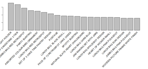
* The most frequent items should be the same as our results in Figure 3.
* Looking at the size of the transactions: 2247 transactions were for just 1 item, 1177 transactions for 2 items, all the way up to the biggest transaction: 1 transaction for 420 items. This indicates that most customers buy a small number of items in each transaction.
* The distribution of the data is right skewed.
Let’s have a look at the item frequency plot, which should be in aligned with Figure 3.
itemFrequencyPlot(tr, topN=20, type='absolute')
Create some rules
-
* We use the Apriori algorithm in Arules library to mine frequent itemsets and association rules. The algorithm employs level-wise search for frequent itemsets.
* We pass supp=0.001 and conf=0.8 to return all the rules that have a support of at least 0.1% and confidence of at least 80%.
* We sort the rules by decreasing confidence.
Have a look at the summary of the rules:
rules <- apriori(tr, parameter = list(supp=0.001, conf=0.8))
rules <- sort(rules, by='confidence', decreasing = TRUE)
summary(rules)
set of 89697 rules

rule length distribution (lhs + rhs):sizes
    2     3     4     5     6     7     8     9    10
  103  3206  9909 26451 31144 14599  3464   700   121

   Min. 1st Qu.  Median    Mean 3rd Qu.    Max.
  2.000   5.000   6.000   5.641   6.000  10.000

summary of quality measures:
    support           confidence          lift             count
 Min.   :0.001036   Min.   :0.8000   Min.   :  8.711   Min.   : 20.00
 1st Qu.:0.001088   1st Qu.:0.8333   1st Qu.: 19.052   1st Qu.: 21.00
 Median :0.001192   Median :0.8750   Median : 24.495   Median : 23.00
 Mean   :0.001382   Mean   :0.8827   Mean   : 49.558   Mean   : 26.67
 3rd Qu.:0.001503   3rd Qu.:0.9231   3rd Qu.: 42.265   3rd Qu.: 29.00
 Max.   :0.018242   Max.   :1.0000   Max.   :622.452   Max.   :352.00

mining info:
 data ntransactions support confidence
   tr         19296   0.001        0.8
The summary of the rules gives us some very interesting information:
-
* The number of rules: 89,697.
* The distribution of rules by length: a length of 6 items has the most rules.
* The summary of quality measures: ranges of support, confidence, and lift.
* The information on data mining: total data mined, and the minimum parameters we set earlier.
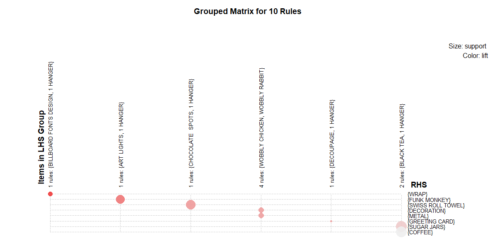
We have 89,697 rules. I don’t want to print them all, so let’s inspect the top 10.
inspect(rules[1:10])
     lhs                         rhs                support     confidence
[1]  {WOBBLY CHICKEN}         => {DECORATION}       0.001451078 1
[2]  {WOBBLY CHICKEN}         => {METAL}            0.001451078 1
[3]  {DECOUPAGE}              => {GREETING CARD}    0.001191957 1
[4]  {BILLBOARD FONTS DESIGN} => {WRAP}             0.001502902 1
[5]  {WOBBLY RABBIT}          => {DECORATION}       0.001762023 1
[6]  {WOBBLY RABBIT}          => {METAL}            0.001762023 1
[7]  {BLACK TEA}              => {SUGAR JARS}       0.002332090 1
[8]  {BLACK TEA}              => {COFFEE}           0.002332090 1
[9]  {CHOCOLATE  SPOTS}       => {SWISS ROLL TOWEL} 0.002176617 1
[10] {ART LIGHTS}             => {FUNK MONKEY}      0.002021144 1
     lift      count
[1]  385.92000 28
[2]  385.92000 28
[3]  344.57143 23
[4]  622.45161 29
[5]  385.92000 34
[6]  385.92000 34
[7]  212.04396 45
[8]   61.06329 45
[9]  410.55319 42
[10] 494.76923 39
The interpretation is pretty straightforward:
-
* 100% customers who bought “WOBBLY CHICKEN” also bought “DECORATION”.
* 100% customers who bought “BLACK TEA” also bought “SUGAR JAR”.
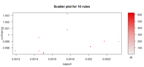
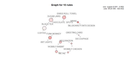
And plot these top 10 rules.
topRules <- rules[1:10]
plot(topRules)
plot(topRules, method="graph")
plot(topRules, method = "grouped")
Summary
In this post, we have learned how to perform Market Basket Analysis in R and how to interpret the results. If you want to implement them in Python, Mlxtend is a Python library that has an implementation of the Apriori algorithm for this sort of application. You can find an introduction tutorial here.
If you would like the R Markdown file used to make this blog post, you can find here.
Reference
- R and Data Mining
