Many of the methods used in time series analysis and forecasting have been around for quite some time but have taken a back seat to machine learning techniques in recent years. Nevertheless, time series analysis and forecasting are useful tools in any data scientist’s toolkit. Some recent time series-based competitions have recently appeared on kaggle, such as one hosted by Wikipedia where competitors are asked to forecast web traffic to various pages of the site. As an economist, I have been working with time series data for many years; however, I was largely unfamiliar with (and a bit overwhelmed by) R’s functions and packages for working with them. From the base ts objects to a whole host of other packages like xts, zoo, TTR, forecast, quantmod and tidyquant, R has a large infrastructure supporting time series analysis. I decided to put together a guide for myself in Rmarkdown. I plan on sharing this as I go in a series of blog posts. In part 1, I’ll discuss the fundamental object in R – the ts object.
The Time Series Object
In order to begin working with time series data and forecasting in R, you must first acquaint yourself with R’s ts object. The ts object is a part of base R. Other packages such as xts and zoo provide other APIs for manipulating time series objects. I’ll cover those in a later part of this guide.
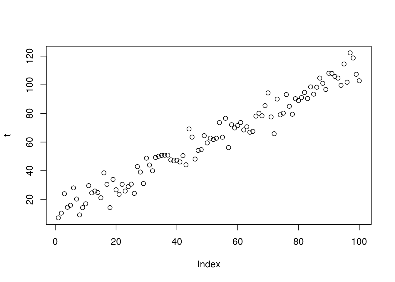
Here we create a vector of simulated data that could potentially represent some real-world time-based data generation process. It is simply a sequence from 1 to 100 scaled up by 10 to avoid negatives and with some random normal noise added to it. We can use R’s base plot() function to see what it looks like:
set.seed(123)
t <- seq(from = 1, to = 100, by = 1) + 10 + rnorm(100, sd = 7)
plot(t)
This could potentially represent some time series, with time represented along the x-axis. However, it’s hard to tell. The x-axis is simply an index from 1 to 100 in this case.
A vector object such as t above can easily be converted to a time series object using the ts() function. The ts() function takes several arguments, the first of which, x, is the data itself. We can look at all of the arguments of ts() using the args() function:
args(ts)
function (data = NA, start = 1, end = numeric(), frequency = 1,
    deltat = 1, ts.eps = getOption("ts.eps"), class = if (nseries >
        1) c("mts", "ts", "matrix") else "ts", names = if (!is.null(dimnames(data))) colnames(data) else paste("Series",
        seq(nseries)))
NULL
To begin, we will focus on the first four arguments – data, start, end and frequency. The data argument is the data itself (a vector or matrix). The start and end arguments allow us to provide a start date and end date for the series. Finally the frequency argument lets us specify the number of observations per unit of time. For example, if we had monthly data, we would use 12 for the frequency argument, indicating that there are 12 months in the year.
Let’s assume our generated data is quarterly data that starts in the first quarter of 2000. We would turn it into a ts object as below. We specify the start argument as a two element vector. The first element is the year and the second element is the observation of that year in which the data start. Because our data is quarterly, we use 4 for the frequency argument.
tseries <- ts(t, start = c(2000, 1), frequency = 4)
print(tseries)
           Qtr1       Qtr2       Qtr3       Qtr4
2000   7.076670  10.388758  23.910958  14.493559
2001  15.905014  28.005455  20.226413   9.144571
2002  14.192030  16.880366  29.568573  24.518697
2003  25.805400  24.774779  21.109112  38.508392
2004  30.484953  14.233680  33.909491  26.690460
2005  23.525234  30.474176  25.817969  28.897761
2006  30.624725  24.193147  42.864509  39.073612
2007  31.033041  48.776704  43.985250  39.934500
2008  49.265880  50.146934  50.751068  50.820482
2009  50.877424  47.566618  46.858261  47.336703
2010  46.137051  50.544579  44.142226  69.182692
2011  63.455734  48.138240  54.179806  54.733413
2012  64.459756  59.416417  62.773230  61.800173
2013  62.699907  73.580216  63.419603  76.615294
2014  56.158730  72.092296  69.866980  71.511591
2015  73.657476  68.483736  70.667548  66.869972
2016  67.497461  78.124700  80.137468  78.371030
2017  85.455872  94.350593  77.562782  65.835818
2018  90.040170  79.035595  80.183940  93.179000
2019  85.006589  79.454976  90.269124  89.027760
2020  91.040349  94.696963  90.405380  98.510636
2021  93.456594  98.322474 104.677873 101.046270
2022  96.718479 108.041653 107.954527 105.838779
2023 104.671122  99.604657 114.524567 101.798183
2024 122.311331 118.728274 107.350097 102.815054
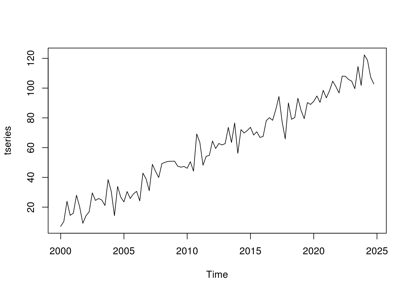
plot(tseries)
Notice that now when we plot the data, R recognizes that it is a ts object and plots the data as a line with dates along the x-axis.
Aside from creating ts objects containing a single series of data, we can also create ts objects that contain multiple series. We can do this by passing a matrix rather than a vector to the x argument of ts().
set.seed(123)
seq <- seq(from = 1, to = 100, by = 1) + 10
ts1 <- seq + rnorm(100, sd = 5)
ts2 <- seq + rnorm(100, sd = 12)
ts3 <- seq^2 + rnorm(100, sd = 300)
tsm <- cbind(ts1, ts2, ts3)
tsm <- ts(tsm, start=c(2000, 1), frequency = 4)
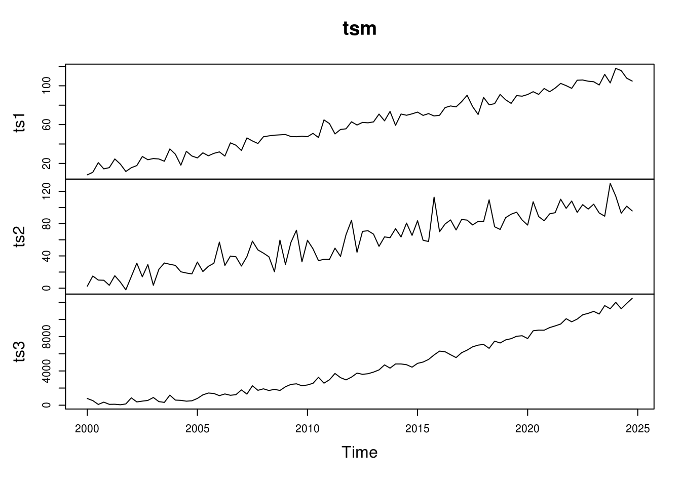
plot(tsm)
Now when we plot the ts object, R automatically facets the plot.
At this point, I should mention what really happens when we call the plot() function on a ts object. R recognizes when the x argument is a ts object and actually calls the plot.ts() function under the hood. We can verify this by using it directly. Notice that it produces an identical graph.
plot.ts(tsm)
The plot.ts() function has different arguments geared towards time series objects. We can look at these again using the args() function.
args(plot.ts)
function (x, y = NULL, plot.type = c("multiple", "single"), xy.labels,
    xy.lines, panel = lines, nc, yax.flip = FALSE, mar.multi = c(0,
        5.1, 0, if (yax.flip) 5.1 else 2.1), oma.multi = c(6,
        0, 5, 0), axes = TRUE, ...)
NULL
Notice that it has an argument called plot.type that lets us indicate whether we want our plot to be faceted (multiple) or single-panel (single). Although in the case of our data above we would not want to plot all three series on the same panel given the difference in scale for ts3, it can be done quite easily.
I am not going to go in-depth into using R’s base plotting capability. Although it is perfectly fine, I strongly prefer to use ggplot2 as well as the ggplot-based graphing functions available in Rob Hyndman’s forecast package. We will discuss these in later parts of this guide.
Convenience Functions for Time Series
There are several useful functions for use with ts objects that can make programming easier. These are window(), start(), end(), and frequency(). These are fairly self-explanatory. The window function is a quick and easy way to obtain a slice of a time series object. For example, look again at our object tseries. Assume that we wanted only the data from the first quarter of 2000 to the last quarter of 2012. We can do so using window():
tseries_sub <- window(tseries, start=c(2000, 1), end=c(2012,4))
print(tseries_sub)
          Qtr1      Qtr2      Qtr3      Qtr4
2000  7.076670 10.388758 23.910958 14.493559
2001 15.905014 28.005455 20.226413  9.144571
2002 14.192030 16.880366 29.568573 24.518697
2003 25.805400 24.774779 21.109112 38.508392
2004 30.484953 14.233680 33.909491 26.690460
2005 23.525234 30.474176 25.817969 28.897761
2006 30.624725 24.193147 42.864509 39.073612
2007 31.033041 48.776704 43.985250 39.934500
2008 49.265880 50.146934 50.751068 50.820482
2009 50.877424 47.566618 46.858261 47.336703
2010 46.137051 50.544579 44.142226 69.182692
2011 63.455734 48.138240 54.179806 54.733413
2012 64.459756 59.416417 62.773230 61.800173
The start() function returns the start date of a ts object, end() gives the end date, and frequency() returns the frequency of a given time series:
start(tsm)
end(tsm)
frequency(tsm)
## [1] 2000    1
## [1] 2024    4
## [1] 4
That’s all for now. In Part 2, we’ll dive into some of the many transformation functions for working with time series in R. See you then.


