Support vector machines are a famous and a very strong classification technique which does not use any sort of probabilistic model like any other classifier but simply generates hyperplanes or simply putting lines, to separate and classify the data in some feature space into different regions.
Support Vector Classifiers are majorly used for solving binary classification problems where we only have 2 class labels say \(Y=[−1,1]\) and a bunch of predictors \(X_i\). And what SVM does is that it generates hyperplanes which in simple terms are just straight lines or planes or are non-linear curves, and these lines are used to separate the data or divide the data into 2 categories or more depending on the type of classification problem.
Another important concept in SVM is of maximal margin classifiers.What it means is that amongst a set of separating hyperplanes SVM aims at finding the one which maximizes the margin \(M\). This simply means that we want to maximize the gap or the distance between the 2 classes from the decision boundary(separating plane). This concept of separating data linearly into 2 different classes using a linear separator or a straight linear line is called linear separability.
The term support vectors in SVM are the data points or training examples which are used to define or maximizing the margin. The support vectors are the points which are close to the decision boundary or on the wrong side of the boundary.
But it is often encountered that linear separators and non-linear decision boundaries fail because of the non-linear interactions in the data and the nonlinear dependence between the features in feature space.
In this tutorial I am going to talk about generating non-linear decision boundaries which is able to separate non linear data using radial kernel support vector classifier.
So how do we separate non-linear data?
The trick here is by doing feature expansion. So the way we solve this problem is by doing a non-linear transformation on the features \(X_i\) and converting them to a higher dimensional space(say 2-D to 3-D space) called a feature space. Now by this transformation, we are able to separate non-linear data using a non-linear decision boundary.
One famous and most general way of adding non-linearities in a model to capture non-linear interactions is by simply using higher degree terms such as square and cubic polynomial terms.
$$y_i = \beta_0+ \beta_1X_1 + \beta_2X_1^2+ \beta_3X_2 + \beta_4X_2^2 + \beta_5X_2^3…. = 0 $$
Above equation is the equation of the non-linear hyperplane which is generated if we use higher degree polynomial terms to fit the data to get a non-linear decision boundary.
What we are actually doing is that we are fitting an SVM is an enlarged space. We enlarge the space of features by fitting non-linear functions in predictors \(X_i\). But the problem with polynomials is that in higher dimension i.e when having lots of predictors it gets wild and generally overfits at higher degrees of the polynomial.
Hence there is another elegant way of adding non-linearities in SVM is by the use of Kernel trick.
Kernel function
Kernel function is a function of form–
$$K(x,y) = (1 + \sum_{j=1}^{p} x_{ij} y_{ij})^d $$ , where d is the degree of polynomial.
Now the type of Kernel function we are going to use here is a Radial kernel.It is of form-
$$K(x,y) = exp(-\gamma \sum_{j=1}^{p}(x_{ij} – y_{ij})^2 )$$ , and \(\gamma\) here is a tuning parameter which accounts for the smoothness of the decision boundary and controls the variance of the model.
If \(\gamma\) is very large then we get quiet fluctuating and wiggly decision boundaries which accounts for high variance and overfitting.
If \(\gamma\) is small, the decision line or boundary is smoother and has low variance.
So now the equation of the support vector classifier becomes —
$$f(x) = \beta_0 + \sum_{i \in S} \alpha_i K(x_i,y_i)$$
Here S are the support vectors and \(\alpha\) is simply a weight value which is non-zero for all support vectors and otherwise 0.
Implementation in R
I will use the ‘e1071’ package to implement Radial SVM in R.
require(e1071)
require(ElemStatLearn)#package containing the dataset

#Loading the data
attach(mixture.example) #is just a simulated mixture data with 200 rows and 2 classes
names(mixture.example)
## [1] "x"        "y"        "xnew"     "prob"     "marginal" "px1"
## [7] "px2"      "means"
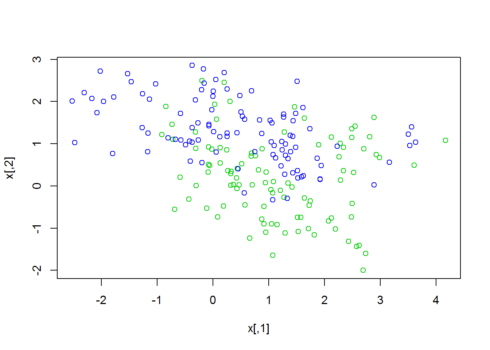
The following data is also 2-D, so let’s plot it. The 2 different colored points represent the different classes.
plot(x,col=y+3)
#converting data to a data frame
data<-data.frame(y=factor(y),x)
head(data)
##   y          X1         X2
## 1 0  2.52609297  0.3210504
## 2 0  0.36695447  0.0314621
## 3 0  0.76821908  0.7174862
## 4 0  0.69343568  0.7771940
## 5 0 -0.01983662  0.8672537
## 6 0  2.19654493 -1.0230141
Now let’s fit a Radial kernel using svm() function.
Radialsvm=svm(factor(y) ~ .,data=data,kernel="radial",cost=5,scale=F)
Radialsvm
##
## Call:
## svm(formula = factor(y) ~ ., data = data, kernel = "radial",
##     cost = 5, scale = F)
##
##
## Parameters:
##    SVM-Type:  C-classification
##  SVM-Kernel:  radial
##        cost:  5
##       gamma:  0.5
##
## Number of Support Vectors:  103
The output of the model is a non-linear decision boundary and the values of the tuning parameters \(C,\gamma\) and the number of support vectors too.
Let’s generate a Confusion matrix to check the model’s performance.
#Confusion matrix to ckeck the accuracy
table(predicted=Radialsvm$fitted,actual=data$y)
##          actual
## predicted  0  1
##         0 76 10
##         1 24 90
let’s calculate the mis-classification rate–
#misclassification Rate
mean(Radialsvm$fitted!=data$y)*100 #17% wrong predictions
## [1] 17%
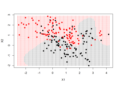
Now let’s create a grid and make a prediction on those grid values and also generate a plot with the decision boundary.
xgrid=expand.grid(X1=px1,X2=px2) #generating grid points

ygrid=predict(Radialsvm,newdata = xgrid) #ygird consisting of predicted Response values

#lets plot the non linear decision boundary
plot(xgrid,col=as.numeric(ygrid),pch=20,cex=0.3)
points(x,col=y+1,pch=19)
#we can see that the decision boundary is non linear
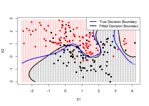
Now we can also improve the above plot,by actually including the decision boundary using the contour() function.
Now the code below is a little bit confusing , so i urge the readers to use the help documentation of the below used functions-
func = predict(Radialsvm,xgrid,decision.values = TRUE)
func=attributes(func)$decision #to pull out all the attributes and use decision attr

#let's again plot the decision boundary
plot(xgrid,col=as.numeric(ygrid),pch=20,cex=0.3)
points(x,col=y+1,pch=19)
?coutour #to search more on using this function
contour(px1,px2,matrix(func,69,99),level=0,add=TRUE,lwd=3) #adds the non linear decision boundary
contour(px1,px2,matrix(prob,69,99),level=0.5,add=T,col="blue",lwd=3)#this is the true decision boundary i.e Bayes decision boundary
legend("topright",c("True Decision Boundary","Fitted Decision Boundary"),lwd=3,col=c("blue","black"))
Gives output :
The above plot shows us the tradeoffs between the true Bayes decision boundary and the fitted decision boundary generated by the radial kernel by learning from data. Both look quite similar and seems that SVM has done a good functional approximation of the actual true underlying function.
Conclusion
Radial kernel support vector machine is a good approach when the data is not linearly separable. The idea behind generating non-linear decision boundaries is that we need to do some nonlinear transformations on the features X\(_i\) which transforms them into a higher dimensional space. We do this non-linear transformation using the Kernel trick. Now the performance of SVM is influenced by the values of the tuning parameters. Now there are 2 Tuning parameters in the SVM i.e the regularization parameter \(C\) and \(\gamma\). We can implement cross-validation to find the best values of both these tuning parameters which affect our classifier’s \(C(X)\) performance. Another way of finding the best value for these hyper-parameters is by using certain optimization techniques such as Bayesian Optimization.
Hope you guys liked the article and make sure to like and share it with your peers.
I am sure that it is motivating enough to get you started with generating your own support vector classifier and use it’s amazing power to generate non-linear decision boundaries and learn non-linear interactions from data.


