Analytical challenges in multivariate data analysis and predictive modeling include identifying redundant and irrelevant variables. A recommended analytics approach is to first address the redundancy; which can be achieved by identifying groups of variables that are as correlated as possible among themselves and as uncorrelated as possible with other variable groups in the same data set. On the other hand, relevancy is about potential predictor variables and involves understanding the relationship between the target variable and input variables.
Multiple correspondence analysis (MCA) is a multivariate data analysis and data mining tool for finding and constructing a low-dimensional visual representation of variable associations among groups of categorical variables. Variable clustering as a tool for identifying redundancy is often applied to get a first impression of variable associations and multivariate data structure.
The motivations of this post are to illustrate the applications of: 1) preparing input variables for analysis and predictive modeling, 2) MCA as a multivariate exploratory data analysis and categorical data mining tool for business insights of customer churn data, and 3) variable clustering of categorical variables for the identification of redundant variables.
Customer churn data in this analysis:
Customer attrition is a metrics businesses use to monitor and quantify the loss of customers and/or clients for various reasons. The data set includes customer-level demographic, account and services information including monthly charge amounts and length of service with the company. Customers who left the company for competitors (Yes) or staying with the company (No) have been identified in the last column labeled churn.
Load Packages
require(caret)
require(plyr)
require(car)
require(dplyr)
require(reshape2)
theme_set(theme_bw(12))
Import and Pre-process Data
The data set used in this post was obtained from the watson-analytics-blog site. Click the hyperlink “Watson Analytics Sample Dataset – Telco Customer Churn” to download the file “WA_Fn-UseC_-Telco-Customer-Churn.csv”.
setwd("path to the location  of your copy of the saved csv data file")

churn <- read.table("WA_Fn-UseC_-Telco-Customer-Churn,csv", sep=",", header=TRUE)
## inspect data dimensions and structure
str(churn)
## 'data.frame':    7043 obs. of  21 variables:
##  $ customerID      : Factor w/ 7043 levels "0002-ORFBO","0003-MKNFE",..: 5376 3963 2565 5536 6512 6552 1003 4771 5605 4535 ...
##  $ gender          : Factor w/ 2 levels "Female","Male": 1 2 2 2 1 1 2 1 1 2 ...
##  $ SeniorCitizen   : int  0 0 0 0 0 0 0 0 0 0 ...
##  $ Partner         : Factor w/ 2 levels "No","Yes": 2 1 1 1 1 1 1 1 2 1 ...
##  $ Dependents      : Factor w/ 2 levels "No","Yes": 1 1 1 1 1 1 2 1 1 2 ...
##  $ tenure          : int  1 34 2 45 2 8 22 10 28 62 ...
##  $ PhoneService    : Factor w/ 2 levels "No","Yes": 1 2 2 1 2 2 2 1 2 2 ...
##  $ MultipleLines   : Factor w/ 3 levels "No","No phone service",..: 2 1 1 2 1 3 3 2 3 1 ...
##  $ InternetService : Factor w/ 3 levels "DSL","Fiber optic",..: 1 1 1 1 2 2 2 1 2 1 ...
##  $ OnlineSecurity  : Factor w/ 3 levels "No","No internet service",..: 1 3 3 3 1 1 1 3 1 3 ...
##  $ OnlineBackup    : Factor w/ 3 levels "No","No internet service",..: 3 1 3 1 1 1 3 1 1 3 ...
##  $ DeviceProtection: Factor w/ 3 levels "No","No internet service",..: 1 3 1 3 1 3 1 1 3 1 ...
##  $ TechSupport     : Factor w/ 3 levels "No","No internet service",..: 1 1 1 3 1 1 1 1 3 1 ...
##  $ StreamingTV     : Factor w/ 3 levels "No","No internet service",..: 1 1 1 1 1 3 3 1 3 1 ...
##  $ StreamingMovies : Factor w/ 3 levels "No","No internet service",..: 1 1 1 1 1 3 1 1 3 1 ...
##  $ Contract        : Factor w/ 3 levels "Month-to-month",..: 1 2 1 2 1 1 1 1 1 2 ...
##  $ PaperlessBilling: Factor w/ 2 levels "No","Yes": 2 1 2 1 2 2 2 1 2 1 ...
##  $ PaymentMethod   : Factor w/ 4 levels "Bank transfer (automatic)",..: 3 4 4 1 3 3 2 4 3 1 ...
##  $ MonthlyCharges  : num  29.9 57 53.9 42.3 70.7 ...
##  $ TotalCharges    : num  29.9 1889.5 108.2 1840.8 151.7 ...
##  $ Churn           : Factor w/ 2 levels "No","Yes": 1 1 2 1 2 2 1 1 2 1
The raw data set contains 7043 records and 21 variables. Looking at the data structure, some data columns need recoding. For instance, changing values from “No phone service” and “No internet service” to “No”, for consistency. The following code statements are to recode those observations and more.
## recode selected observations
churn$MultipleLines <- as.factor(mapvalues(churn$MultipleLines,
                                           from=c("No phone service"),
                                           to=c("No")))

churn$InternetService <- as.factor(mapvalues(churn$InternetService,
                                             from=c("Fiber optic"),
                                             to=c("Fiberoptic")))

churn$PaymentMethod <- as.factor(mapvalues(churn$PaymentMethod,
                                           from=c("Credit card (automatic)","Electronic check","Mailed check",
"Bank transfer (automatic)"),
                                           to=c("Creditcard","Electronicheck","Mailedcheck","Banktransfer")))

churn$Contract <- as.factor(mapvalues(churn$Contract,
                                      from=c("Month-to-month",
                                             "Two year", "One year"),
                                      to=c("MtM","TwoYr", "OneYr")))


cols_recode1 <- c(10:15)
for(i in 1:ncol(churn[,cols_recode1])) {
        churn[,cols_recode1][,i] <- as.factor(mapvalues
                                              (churn[,cols_recode1][,i], from =c("No internet service"),to=c("No")))
}
Besides, values in the SeniorCitizen column were entered as 0 and 1. Let’s recode this variable as “No” and “Yes”, respectively, for consistency.
churn$SeniorCitizen <- as.factor(mapvalues(churn$SeniorCitizen,
                                      from=c("0","1"),
                                      to=c("No", "Yes")))
Exclude the consumer id and total charges columns from data analysis.
cols_drop <- c(1, 20)
churn <- churn[,-cols_drop]
Let’s do summary statistics of the two numerical variables to see distribution of the data.
summary(churn$MonthlyCharges)
##    Min. 1st Qu.  Median    Mean 3rd Qu.    Max.
##   18.25   35.50   70.35   64.76   89.85  118.80
summary(churn$tenure)
##    Min. 1st Qu.  Median    Mean 3rd Qu.    Max.
##    0.00    9.00   29.00   32.37   55.00   72.00
On the basis of the data distributions above, values in the tenure and monthly charges numerical columns could be coerced to a 3-level categorical value as follows.
churn$tenure <- as.factor(car::recode(churn$tenure, "1:9 = 'ShortTenure';
                               9:29 = 'MediumTenure'; else = 'LongTenure'"))

churn$MonthlyCharges <- as.factor(car::recode(churn$MonthlyCharges, "1:35 = 'LowCharge';35:70 = 'MediumCharge'; else = 'HighCharge'"))
It’s time to check for missing values in the pre-processed data set.
mean(is.na(churn))
## [1] 0
There are no missing values. How about the category levels of each variable?
## check for factor levels in each column
nfactors <- apply(churn, 2, function(x) nlevels(as.factor(x)))
nfactors
##           gender    SeniorCitizen          Partner       Dependents
##                2                2                2                2
##           tenure     PhoneService    MultipleLines  InternetService
##                3                2                2                3
##   OnlineSecurity     OnlineBackup DeviceProtection      TechSupport
##                2                2                2                2
##      StreamingTV  StreamingMovies         Contract PaperlessBilling
##                2                2                3                2
##    PaymentMethod   MonthlyCharges            Churn
##                4                3                2
Now, the data set is ready for analysis.
Partitioning the raw data into 70% training and 30% testing data sets
inTrain <- createDataPartition(churn$Churn, p=0.7, list=FALSE)
## set random seed to make reproducible results
set.seed(324)
training <- churn[inTrain,]
testing <- churn[-inTrain,]
Check for the dimensions of the training and testing data sets
dim(training) ; dim(testing)
## [1] 4931   19
## [1] 2112   19
As expected, the training data set contains 4931 observations and 19 columns, whereas the testing data set contains 2112 observations and 19 columns.
Multiple Correspondence Analysis (MCA)
Invoke the FactoMiner & factoextra packages.
require(FactoMineR)
require(factoextra)
res.mca <- MCA(training, quali.sup=c(17,19), graph=FALSE)
fviz_mca_var(res.mca, repel=TRUE)
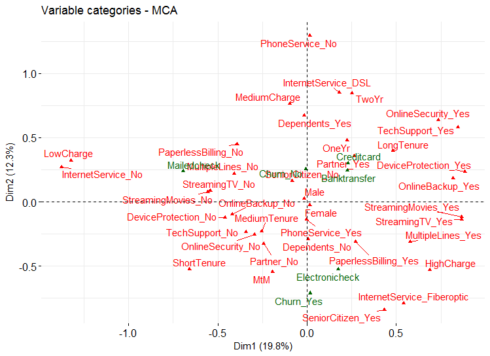
A general guide to extrapolating from the figure above for business insights would be to observe and make a note as to how close input variables are to the target variable and to each other. For instance, customers with month to month contract, those with fiber optic internet service, senior citizens, customers with high monthly charges, single customers or customers with no dependents, those with paperless billing are being related to a short tenure with the company and a propensity of risk to churn.
On the other hand, customers with 1 – 2 years contract, those with DSL internet service, younger customers, those with low monthly charges, customers with multiple lines, online security and tech support services are being related to a long tenure with the company and a tendency to stay with company.
Variable Clustering
Load the ClustOfVar package and the hclustvar function produces a tree of variable groups. A paper detailing the ClustOfVar package is here
require(ClustOfVar)
# run variable clustering excluding the target variable (churn)
variable_tree <- hclustvar(X.quali = training[,1:18])
#plot the dendrogram of variable groups
plot(variable_tree)
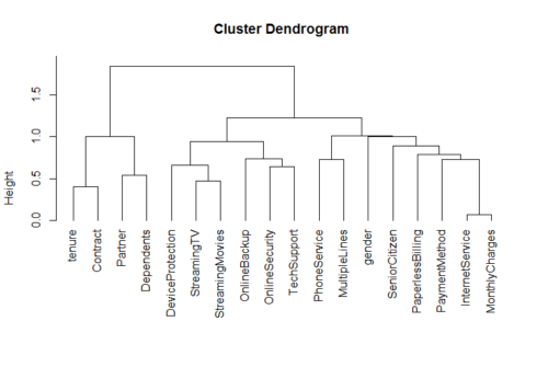
Here is a tree of categorical variable groups.

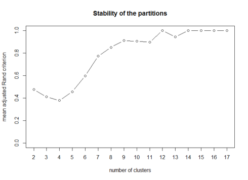
The dendrogram suggests that the 18 input variables can be combined into approximately 7 – 9 groups of variables. That is one way of going about it. The good news is that the ClusofVar package offers a function to cut the cluster into any number of desired groups (clusters) of variables. So, the syntax below will run 25 bootstrap samples of the trees to produce a plot of stability of variable cluster partitions.
# requesting for 25 bootstrap samplings and a plot
stability(variable_tree, B=25)

The plot of stability of variable cluster partitions suggests approximately a 7 to 9-cluster solution. The syntax below will list a consensus list of 9-clusters along with the variables names included in each cluster.
## cut the variable tree into 9(?) groups of variables
clus <- cutreevar(variable_tree,9)
## print the list of variables in each cluster groups
print(clus$var)
## $cluster1
##        squared loading
## gender               1
##
## $cluster2
##               squared loading
## SeniorCitizen               1
##
## $cluster3
##            squared loading
## Partner          0.7252539
## Dependents       0.7252539
##
## $cluster4
##               squared loading
## tenure              0.7028741
## Contract            0.7162027
## PaymentMethod       0.4614923
##
## $cluster5
##               squared loading
## PhoneService        0.6394947
## MultipleLines       0.6394947
##
## $cluster6
##                 squared loading
## InternetService       0.9662758
## MonthlyCharges        0.9662758
##
## $cluster7
##                squared loading
## OnlineSecurity       0.5706136
## OnlineBackup         0.4960295
## TechSupport          0.5801424
##
## $cluster8
##                  squared loading
## DeviceProtection       0.5319719
## StreamingTV            0.6781781
## StreamingMovies        0.6796616
##
## $cluster9
##                  squared loading
## PaperlessBilling               1
The 9-clusters and the variable names in each cluster are listed above. The practical guide to minimizing redundancy is to select a cluster representative. However, subject-matter considerations should have a say in the consideration and selection of other candidate representatives of each variable cluster group.
Descriptive statistics of customer churn
what was the overall customer churn rate in the training data set?
# overall customer churn rate
round(prop.table(table(training$Churn))*100,1)
##
##   No  Yes
## 73.5 26.5
The overall customer attrition rate was approximately 26.5%.
Customer churn rate by demography, account and service information
cols_aggr_demog <- c(1:4,6:7,9:14,16)
variable <- rep(names(training[,cols_aggr_demog]),each=4)
demog_counts=c()
for(i in 1:ncol(training[,cols_aggr_demog])) {
    demog_count <- ddply(training, .(training[,cols_aggr_demog][,i],training$Churn), "nrow")
     names(demog_count) <- c("class","Churn","count")
    demog_counts <- as.data.frame(rbind(demog_counts, demog_count))
 }

demog_churn_rate <- as.data.frame(cbind(variable, demog_counts))
demog_churn_rate1 <- dcast(demog_churn_rate, variable + class ~ Churn, value.var="count")
demog_churn_rate2 <- mutate(demog_churn_rate1, churn_rate=round((Yes/(No+Yes)*100)-26.5,1))
demog <- as.data.frame(paste(demog_churn_rate2$variable,demog_churn_rate2$class))
names(demog) <- c("Category")
demog2 <- as.data.frame(cbind(demog,demog_churn_rate2))
cols_aggr_nlev3 <- c(5,8,15,18)
variable <- rep(names(training[,cols_aggr_nlev3]),each=6)
nlev3_counts=c()
for(i in 1:ncol(training[,cols_aggr_nlev3])) {
    nlev3_count <- ddply(training, .(training[,cols_aggr_nlev3][,i],training$Churn), "nrow")
     names(nlev3_count) <- c("class","Churn","count")
    nlev3_counts <- as.data.frame(rbind(nlev3_counts, nlev3_count))
 }

nlev3_churn_rate <- as.data.frame(cbind(variable, nlev3_counts))
nlev3_churn_rate1 <- dcast(nlev3_churn_rate, variable + class ~ Churn, value.var="count")
nlev3_churn_rate2 <- mutate(nlev3_churn_rate1, churn_rate=round((Yes/(No+Yes)*100)-26.5,1))
nlev3 <- as.data.frame(paste(nlev3_churn_rate2$variable,nlev3_churn_rate2$class))
names(nlev3) <- c("Category")
nlev3 <- as.data.frame(cbind(nlev3,nlev3_churn_rate2))
variable <- rep("PaymentMethod",8)
nlev4_count <- ddply(training, .(training[,17],training$Churn), "nrow")
names(nlev4_count) <- c("class","Churn","count")
nlev4_churn_rate <- as.data.frame(cbind(variable, nlev4_count))
nlev4_churn_rate1 <- dcast(nlev4_churn_rate, variable + class ~ Churn, value.var="count")
nlev4_churn_rate2 <- mutate(nlev4_churn_rate1, churn_rate=round((Yes/(No+Yes)*100)-26.5,1))
nlev4 <- as.data.frame(paste(nlev4_churn_rate$variable4,nlev4_churn_rate2$class))
names(nlev4) <- c("Category")
nlev4 <- as.data.frame(cbind(nlev4,nlev4_churn_rate2))
final_agg <- as.data.frame(rbind(demog2, nlev3, nlev4))

ggplot(final_agg, aes(Category, churn_rate, color=churn_rate < 0)) +
    geom_segment(aes(x=reorder(Category, -churn_rate), xend = Category,
                     y = 0, yend = churn_rate),
                 size = 1.1, alpha = 0.7) +
    geom_point(size = 2.5) +
        theme(legend.position="none") +
    xlab("Variable") +
    ylab("Customer Churn (%)") +
    ggtitle("Customer Attrition rate \n Difference from the overall average (%)") +
    theme(axis.text.x=element_text(angle=45, hjust=1)) +
    coord_flip()
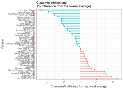
Looking at the figure above, customers with higher than average attrition rates include those with an electronic check, with month to month contracts, with higher monthly charges and paperless billing. On a positive note, customers with low monthly charges, longer period contract, with online security services, with dependents or with partners, those paying with credit card or bank transfer showed a much lower than average rates of attrition.
In conclusion
Variables such as contract length, bill payment method, internet service type and even customer demography appeared to play a role in customer attrition and retention. The next step for this company would be to deploy predictive and prescriptive models that would score prospective customers for the propensity of risk to churn. Hope this post is helpful. Please leave your comments or suggestions below. Ok to networking with the author on LinkedIn.

