To conduct a one-sample t-test in R, we use the syntax t.test(y, mu = 0) where x is the name of our variable of interest and mu is set equal to the mean specified by the null hypothesis.
So, for example, if we wanted to test whether the volume of a shipment of lumber was less than usual (\(\mu_0=39000\) cubic feet), we would run:
set.seed(0)
treeVolume <- c(rnorm(75, mean = 36500, sd = 2000))
t.test(treeVolume, mu = 39000) # Ho: mu = 39000

	One Sample t-test

data:  treeVolume
t = -12.2883, df = 74, p-value < 2.2e-16
alternative hypothesis: true mean is not equal to 39000
95 percent confidence interval:
 36033.60 36861.38
sample estimates:
mean of x
 36447.49
With these simulated data, we see that the current shipment of lumber has a significantly lower volume than we usually see:
t = -12.2883, p-value < 2.2e-16
Paired-Samples T-Tests
To conduct a paired-samples test, we need either two vectors of data, \(y_1\) and \(y_2\), or we need one vector of data with a second that serves as a binary grouping variable. The test is then run using the syntax t.test(y1, y2, paired=TRUE).
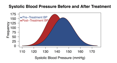
For instance, let’s say that we work at a large health clinic and we’re testing a new drug, Procardia, that’s meant to reduce hypertension. We find 1000 individuals with a high systolic blood pressure (\(\bar{x}=145\)mmHg, \(SD=9\)mmHg), we give them Procardia for a month, and then measure their blood pressure again. We find that the mean systolic blood pressure has decreased to 138mmHg with a standard deviation 8mmHg.
We can visualize this difference with a kernel density plot as:
Here, we would conduct a t-test using:
set.seed(2820)

preTreat <- c(rnorm(1000, mean = 145, sd = 9))
postTreat <- c(rnorm(1000, mean = 138, sd = 8))

t.test(preTreat, postTreat, paired = TRUE)

	Paired t-test

data:  preTreat and postTreat
t = 19.7514, df = 999, p-value < 2.2e-16
alternative hypothesis: true difference in means is not equal to 0
95 percent confidence interval:
 6.703959 8.183011
sample estimates:
mean of the differences
               7.443485
Again, we see that there is a statistically significant difference in means on
t = 19.7514, p-value < 2.2e-16
Independent Samples
The independent-samples test can take one of three forms, depending on the structure of your data and the equality of their variances. The general form of the test is t.test(y1, y2, paired=FALSE). By default, R assumes that the variances of y1 and y2 are unequal, thus defaulting to Welch's test. To toggle this, we use the flag var.equal=TRUE.
In the three examples shown here we’ll test the hypothesis that Clevelanders and New Yorkers spend different amounts monthly eating out. The first example assumes that we have two numeric vectors: one with Clevelanders' spending and one with New Yorkers' spending. The second example uses a binary grouping variable with a single column of spending data. (That is, there is only one column of spending data; however, for each dollar amount, the next column specifies whether it is for a New Yorker or a Clevelander.) Finally, the third example assumes that the variances of the two samples are unequal and uses Welch's test.
Independent-samples t-test where y1 and y2 are numeric:
set.seed(0)

ClevelandSpending <- rnorm(50, mean = 250, sd = 75)
NYSpending <- rnorm(50, mean = 300, sd = 80)

t.test(ClevelandSpending, NYSpending, var.equal = TRUE)

	Two Sample t-test

data:  ClevelandSpending and NYSpending
t = -3.6361, df = 98, p-value = 0.0004433
alternative hypothesis: true difference in means is not equal to 0
95 percent confidence interval:
 -77.1608 -22.6745
sample estimates:
mean of x mean of y
 251.7948  301.7125
Where y1 is numeric and y2 is binary:
spending <- c(ClevelandSpending, NYSpending)
city <- c(rep("Cleveland", 50), rep("New York", 50))

t.test(spending ~ city, var.equal = TRUE)

	Two Sample t-test

data:  spending by city
t = -3.6361, df = 98, p-value = 0.0004433
alternative hypothesis: true difference in means is not equal to 0
95 percent confidence interval:
 -77.1608 -22.6745
sample estimates:
mean in group Cleveland  mean in group New York
               251.7948                301.7125
With equal variances not assumed:
t.test(ClevelandSpending, NYSpending, var.equal = FALSE)

	Welch Two Sample t-test

data:  ClevelandSpending and NYSpending
t = -3.6361, df = 97.999, p-value = 0.0004433
alternative hypothesis: true difference in means is not equal to 0
95 percent confidence interval:
 -77.1608 -22.6745
sample estimates:
mean of x mean of y
 251.7948  301.7125
In each case, we see that the results really don’t differ substantially: our simulated data show that in any case New Yorkers spend more each month at restaurants than Clevelanders do. However, should you want to test for equality of variances in your data prior to running an independent-samples t-test, R offers an easy way to do so with the var.test() function:
var.test(ClevelandSpending, NYSpending)

	F test to compare two variances

data:  ClevelandSpending and NYSpending
F = 1.0047, num df = 49, denom df = 49, p-value = 0.9869
alternative hypothesis: true ratio of variances is not equal to 1
95 percent confidence interval:
 0.5701676 1.7705463
sample estimates:
ratio of variances
          1.004743
Have questions? Post a comment below! Or download the full code used in this example.
