In this post, I will show how to collect data from a webpage and analyze or visualize in R. For this task I will use the rvest package and will get the data from Wikipedia. I got the idea to write this post from Fisseha Berhane.
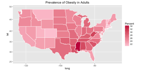
I will gain access to the prevalence of obesity in the US from Wikipedia page, then I will plot it on the map. Let’s begin with loading the required packages.
## LOAD THE PACKAGES ####
library(rvest)
library(ggplot2)
library(dplyr)
library(scales)
Download the data from Wikipedia.
## LOAD THE DATA ####
obesity = read_html("https://en.wikipedia.org/wiki/Obesity_in_the_United_States")

obesity = obesity %>%
     html_nodes("table") %>%
     .[[1]]%>%
     html_table(fill=T)
The first line of code is calling the data from Wikipedia and the second line of codes is transforming the table that we are interested into a data frame in R.
The head of our data.
head(obesity)
State and District of Columbia Obese adults Overweight (incl. obese) adults
1                        Alabama        30.1%                           65.4%
2                         Alaska        27.3%                           64.5%
3                        Arizona        23.3%                           59.5%
4                       Arkansas        28.1%                           64.7%
5                     California        23.1%                           59.4%
6                       Colorado        21.0%                           55.0%
  Obese children and adolescents Obesity rank
1                          16.7%            3
2                          11.1%           14
3                          12.2%           40
4                          16.4%            9
5                          13.2%           41
6                           9.9%           51
The data frame looks good, now we need to clean it from making ready to plot.
## CLEAN THE DATA ####
str(obesity)
# remove the % and make the data numeric
for(i in 2:4){
     obesity[,i] = gsub("%", "", obesity[,i])
     obesity[,i] = as.numeric(obesity[,i])
}
# check data again
str(obesity)
'data.frame':	51 obs. of  5 variables:
 $ State and District of Columbia : chr  "Alabama" "Alaska" "Arizona" "Arkansas" ...
 $ Obese adults                   : chr  "30.1%" "27.3%" "23.3%" "28.1%" ...
 $ Overweight (incl. obese) adults: chr  "65.4%" "64.5%" "59.5%" "64.7%" ...
 $ Obese children and adolescents : chr  "16.7%" "11.1%" "12.2%" "16.4%" ...
 $ Obesity rank                   : int  3 14 40 9 41 51 49 43 22 39 ...

'data.frame':	51 obs. of  5 variables:
 $ State and District of Columbia : chr  "Alabama" "Alaska" "Arizona" "Arkansas" ...
 $ Obese adults                   : num  30.1 27.3 23.3 28.1 23.1 21 20.8 22.1 25.9 23.3 ...
 $ Overweight (incl. obese) adults: num  65.4 64.5 59.5 64.7 59.4 55 58.7 55 63.9 60.8 ...
 $ Obese children and adolescents : num  16.7 11.1 12.2 16.4 13.2 9.9 12.3 14.8 22.8 14.4 ...
 $ Obesity rank                   : int  3 14 40 9 41 51 49 43 22 39 ...
Fix the names of variables by removing the spaces.
names(obesity)
names(obesity) = make.names(names(obesity))
names(obesity)
[1] "State and District of Columbia"  "Obese adults"
[3] "Overweight (incl. obese) adults" "Obese children and adolescents"
[5] "Obesity rank"
[1] "State.and.District.of.Columbia"  "Obese.adults"
[3] "Overweight..incl..obese..adults" "Obese.children.and.adolescents"
[5] "Obesity.rank"
Now, it’s time to load the map data.
# load the map data
states = map_data("state")
str(states)
'data.frame':	15537 obs. of  6 variables:
 $ long     : num  -87.5 -87.5 -87.5 -87.5 -87.6 ...
 $ lat      : num  30.4 30.4 30.4 30.3 30.3 ...
 $ group    : num  1 1 1 1 1 1 1 1 1 1 ...
 $ order    : int  1 2 3 4 5 6 7 8 9 10 ...
 $ region   : chr  "alabama" "alabama" "alabama" "alabama" ...
 $ subregion: chr  NA NA NA NA ...
Merge two datasets (obesity and states) by region, therefore we first need to create a new variable (region) in obesity dataset.
# create a new variable name for state
obesity$region = tolower(obesity$State.and.District.of.Columbia)
Merge the datasets.
states = merge(states, obesity, by="region", all.x=T)
str(states)
'data.frame':	15537 obs. of  11 variables:
 $ region                         : chr  "alabama" "alabama" "alabama" "alabama" ...
 $ long                           : num  -87.5 -87.5 -87.5 -87.5 -87.6 ...
 $ lat                            : num  30.4 30.4 30.4 30.3 30.3 ...
 $ group                          : num  1 1 1 1 1 1 1 1 1 1 ...
 $ order                          : int  1 2 3 4 5 6 7 8 9 10 ...
 $ subregion                      : chr  NA NA NA NA ...
 $ State.and.District.of.Columbia : chr  "Alabama" "Alabama" "Alabama" "Alabama" ...
 $ Obese.adults                   : num  30.1 30.1 30.1 30.1 30.1 30.1 30.1 30.1 30.1 30.1 ...
 $ Overweight..incl..obese..adults: num  65.4 65.4 65.4 65.4 65.4 65.4 65.4 65.4 65.4 65.4 ...
 $ Obese.children.and.adolescents : num  16.7 16.7 16.7 16.7 16.7 16.7 16.7 16.7 16.7 16.7 ...
 $ Obesity.rank                   : int  3 3 3 3 3 3 3 3 3 3 ...
Plot the data
Finally we will plot the prevalence of obesity in adults.
## MAKE THE PLOT ####

# adults
ggplot(states, aes(x = long, y = lat, group = group, fill = Obese.adults)) +
     geom_polygon(color = "white") +
     scale_fill_gradient(name = "Percent", low = "#feceda", high = "#c81f49", guide = "colorbar", na.value="black", breaks = pretty_breaks(n = 5)) +
     labs(title="Prevalence of Obesity in Adults") +
     coord_map()
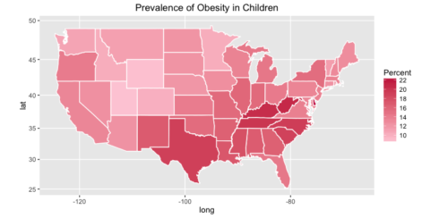
Similarly, we can plot the prevalence of obesity in children.
# children
ggplot(states, aes(x = long, y = lat, group = group, fill = Obese.children.and.adolescents)) +
     geom_polygon(color = "white") +
     scale_fill_gradient(name = "Percent", low = "#feceda", high = "#c81f49", guide = "colorbar", na.value="black", breaks = pretty_breaks(n = 5)) +
     labs(title="Prevalence of Obesity in Children") +
     coord_map()
If you like to show the name of State on the map use the code below to create a new dataset.
statenames = states %>%
     group_by(region) %>%
     summarise(
          long = mean(range(long)),
          lat = mean(range(lat)),
          group = mean(group),
          Obese.adults = mean(Obese.adults),
          Obese.children.and.adolescents = mean(Obese.children.and.adolescents)
 )
After you add this code to ggplot code above
geom_text(data=statenames, aes(x = long, y = lat, label = region), size=3)
That’s all. I hope you learned something useful today.

