The dplyr package, which is one of my favorite R packages, works with in-memory data and with data stored in databases. In this extensive and comprehensive post, I will share my experience on using dplyr to work with databases. The basic functions of dplyr package are covered in another post at DataScience+
Using dplyr with databases has huge advantage when our data is big where loading it to R is impossible or slows down our analytics. If our data resides in a database, rather than loading the whole data to R, we can work with subsets or aggregates of the data that we are interested in. Further, if we have many data files, putting our data in a database, rather than in csv or other format, has better security and is easier to manage.
dplyr is a really powerful package for data manipulation, data exploration and feature engineering in R and if you do not know SQL, it provides the ability to work with databases just within R. Further, dplyr functions are easy to write and read. dplyr considers database tables as data frames and it uses lazy evaluation (it delays the actual operation until necessary and loads data onto R from the database only when we need it) and for someone who knows Spark, the processes and even the functions have similarities.
dplyr supports a couple of databases such as sqlite, mysql and postgresql. In this post, we will see how to work with sqlite database. You can get more information from the dplyr database vignette here.
When people take drugs, if they experience any adverse events, they can report it to the FDA. These data are in public domain and anyone can download them and analyze them. In this post, we will download demography information of the patients, drug they used and for what indication they used it, reaction and outcome. Then, we will put all the datasets in a database and use dplyr to work with the databases.
You can read more about the adverse events data in my previous post.
You can simply run the code below and it will download the adverse events data and create one large dataset, for each category, by merging the various datasets. For demonstration purposes, let’s use the adverse event reports from 2013-2015. The adverse events are released in quarterly data files (a single data file for every category every three months).
Load R Packages
library(dplyr)
library(ggplot2)
library(data.table)
Download adverse events data
 year_start=2013
year_last=2015
for (i in year_start:year_last){
            j=c(1:4)
            for (m in j){
            url1<-paste0("http://www.nber.org/fda/faers/",i,"/demo",i,"q",m,".csv.zip")
                download.file(url1,dest="data.zip") # Demography
                unzip ("data.zip")
            url2<-paste0("http://www.nber.org/fda/faers/",i,"/drug",i,"q",m,".csv.zip")
                download.file(url2,dest="data.zip")   # Drug
                unzip ("data.zip")
            url3<-paste0("http://www.nber.org/fda/faers/",i,"/reac",i,"q",m,".csv.zip")
                download.file(url3,dest="data.zip") # Reaction
                unzip ("data.zip")
            url4<-paste0("http://www.nber.org/fda/faers/",i,"/outc",i,"q",m,".csv.zip")
                download.file(url4,dest="data.zip") # Outcome
                unzip ("data.zip")
            url5<-paste0("http://www.nber.org/fda/faers/",i,"/indi",i,"q",m,".csv.zip")
                download.file(url5,dest="data.zip") # Indication for use
                unzip ("data.zip")
            }
        }
Concatenate the quarterly data files and create single dataset for each category
Demography
filenames <- list.files(pattern="^demo.*.csv", full.names=TRUE)
demography = rbindlist(lapply(filenames, fread,
        select=c("primaryid","caseid","age","age_cod","event_dt",
         "sex","wt","wt_cod","occr_country"),data.table=FALSE))

str(demography)
'data.frame':	3037542 obs. of  9 variables:
 $ primaryid   : int  30375293 30936912 32481334 35865322 37005182 37108102 37820163 38283002 38346784 40096383 ...
 $ caseid      : int  3037529 3093691 3248133 3586532 3700518 3710810 3782016 3828300 3834678 4009638 ...
 $ age         : chr  "44" "38" "28" "45" ...
 $ age_cod     : chr  "YR" "YR" "YR" "YR" ...
 $ event_dt    : int  199706 199610 1996 20000627 200101 20010810 20120409 NA 20020615 20030619 ...
 $ sex         : chr  "F" "F" "F" "M" ...
 $ wt          : num  56 56 54 NA NA 80 102 NA NA 87.3 ...
 $ wt_cod      : chr  "KG" "KG" "KG" "" ...
 $ occr_country: chr  "US" "US" "US" "AR" ...
We see that our demography data has more than 3 million rows and the variables are age, age code, date the event happened, sex, weight, weight code and country where the event happened.
Drug
 filenames <- list.files(pattern="^drug.*.csv", full.names=TRUE)
 drug = rbindlist(lapply(filenames, fread,
        select=c("primaryid","drug_seq","drugname","route"
         ),data.table=FALSE))

str(drug)
'data.frame':	9989450 obs. of  4 variables:
 $ primaryid: chr  "" "" "" "" ...
 $ drug_seq : chr  "" "" "20140601" "U" ...
 $ drugname : chr  "" "" "" "" ...
 $ route    : chr  "" "21060" "" "76273" ...
We can see that the drug data has about ten million rows and among the variables are drug name and route.
Diagnoses/Indications
 filenames <- list.files(pattern="^indi.*.csv", full.names=TRUE)
 indication = rbindlist(lapply(filenames, fread,
        select=c("primaryid","indi_drug_seq","indi_pt"
         ),data.table=FALSE))

str(indication)
'data.frame':	6383312 obs. of  3 variables:
 $ primaryid    : int  8480348 8480354 8480355 8480357 8480358 8480358 8480358 8480359 8480360 8480361 ...
 $ indi_drug_seq: int  1020135312 1020135329 1020135331 1020135333 1020135334 1020135337 1020135338 1020135339 1020135340 1020135341 ...
 $ indi_pt      : chr  "CONTRACEPTION" "SCHIZOPHRENIA" "ANXIETY" "SCHIZOPHRENIA" ...
The indication data has more than six million rows and the variables are primaryid, drug sequence and indication (indication prefered term).
Outcomes
filenames <- list.files(pattern="^outc.*.csv", full.names=TRUE)
outcome = rbindlist(lapply(filenames, fread,
        select=c("primaryid","outc_cod"),data.table=FALSE))

str(outcome)
 'data.frame':	2453953 obs. of  2 variables:
 $ primaryid: int  8480347 8480348 8480350 8480351 8480352 8480353 8480353 8480354 8480355 8480356 ...
 $ outc_cod : chr  "OT" "HO" "HO" "HO" ...
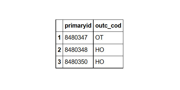
The outcome data has more than two million rows and the variables are primaryid and outcome code (outc_cod).
Reaction (Adverse Event)
filenames <- list.files(pattern="^reac.*.csv", full.names=TRUE)
reaction = rbindlist(lapply(filenames, fread,
           select=c("primaryid","pt"),data.table=FALSE))

str(reaction)
'data.frame':	9288270 obs. of  2 variables:
 $ primaryid: int  8480347 8480348 8480349 8480350 8480350 8480350 8480350 8480350 8480350 8480351 ...
 $ pt       : chr  "ANAEMIA HAEMOLYTIC AUTOIMMUNE" "OPTIC NEUROPATHY" "DYSPNOEA" "DEPRESSED MOOD" ...
So, we see that the adverse events (reaction) data has more than nine million rows and the variables are primaryid and prefered term for adverse event (pt).
Create a database
To create SQLite database in R, we do not need anything, just specifying the path only. We use src_sqlite to connect to an existing sqlite database, and tbl to connect to tables within that database. We can also use src_sqlite to create new SQlite database at the specified path. If we do not specify a path, it will be created in our working directory.
my_database<- src_sqlite("adverse_events", create = TRUE) # create =TRUE creates a new database
Put data in the database
To upload data to the database, we use the dplyr function copy_to. According to the documentation, wherever possible, the new object will be temporary, limited to the current connection to the source. So, we have to change temporary to false to make it permanent.
 copy_to(my_database,demography,temporary = FALSE) # uploading demography data
copy_to(my_database,drug,temporary = FALSE)       # uploading drug data
copy_to(my_database,indication,temporary = FALSE) # uploading indication data
copy_to(my_database,reaction,temporary = FALSE)   # uploading reaction data
copy_to(my_database,outcome,temporary = FALSE)     #uploading outcome data
Now, I have put all the datasets in the “adverse_events” database. I can query it and do analytics I want.
Connect to database
my_db <- src_sqlite("adverse_events", create = FALSE)
              # create is false now because I am connecting to an existing database
List the tables in the database
src_tbls(my_db)

    "demography" "drug" "indication" "outcome" "reaction" "sqlite_stat1"
Querying the database
We use the same dplyr verbs that we use in data manipulation to work with databases. dplyr translates the R code we write to SQL code. We use tbl to connect to tables within the database.
demography = tbl(my_db,"demography" )

class(demography)
tbl_sqlite" "tbl_sql" "tbl"

head(demography,3)
US = filter(demography, occr_country=='US') # Filtering demography of patients from the US
We can see the query dplyr has generated:
US$query
 SELECT "primaryid", "caseid", "age", "age_cod", "event_dt", "sex", "wt", "wt_cod", "occr_country"
FROM "demography"
WHERE "occr_country" = 'US'
We can also see how the database plans to execute the query:
explain(US)

SELECT "primaryid", "caseid", "age", "age_cod", "event_dt", "sex", "wt", "wt_cod", "occr_country"
FROM "demography"
WHERE "occr_country" = 'US'
  selectid order from                detail
1        0     0    0 SCAN TABLE demography
Let’s similarly connect to the other tables in the database.
drug = tbl(my_db,"drug" )
indication = tbl(my_db,"indication" )
outcome = tbl(my_db,"outcome" )
reaction = tbl(my_db,"reaction" )
It is very interesting to note that dplyr delays the actual operation until necessary and loads data onto R from the database only when we need it. When we use actions such as collect(), head(), count(), etc, the commands are executed.
While we can use head() on database tbls, we can’t find the last rows without executing the whole query.
head(indication,3)
tail(indication,3)
Error: tail is not supported by sql sources
dplyr verbs (select, arrange, filter, mutate, summarize, rename) on the tables from the database
We can pipe dplyr operations together with %>% from the magrittr R package. The pipeline %>% takes the output from the left-hand side of the pipe as the first argument to the function on the right hand side.
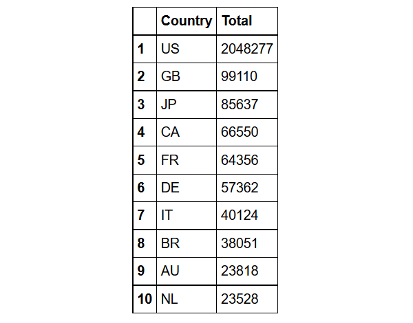
Find the top ten countries with the highest number of adverse events
demography%>%group_by(Country= occr_country)%>%
           summarize(Total=n())%>%
           arrange(desc(Total))%>%
           filter(Country!='')%>% head(10)
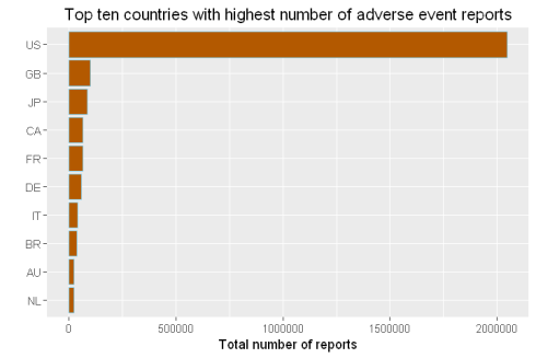
We can also include ggplot in the chain:
demography%>%group_by(Country= occr_country)%>% #grouped by country
           summarize(Total=n())%>%    # found the count for each country
           arrange(desc(Total))%>%    # sorted them in descending order
           filter(Country!='')%>%     # removed reports that does not have country information
           head(10)%>%                   # took the top ten
           mutate(Country = factor(Country,levels = Country[order(Total,decreasing =F)]))%>%
        ggplot(aes(x=Country,y=Total))+geom_bar(stat='identity',color='skyblue',fill='#b35900')+
           xlab("")+ggtitle('Top ten countries with highest number of adverse event reports')+
           coord_flip()+ylab('Total number of reports')
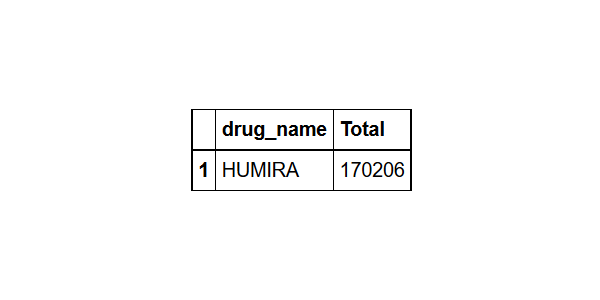
Find the most common drug
drug%>%group_by(drug_name= drugname)%>% #grouped by drug_name
           summarize(Total=n())%>%    # found the count for each drug name
           arrange(desc(Total))%>%    # sorted them in descending order
           head(1)                   # took the most frequent drug
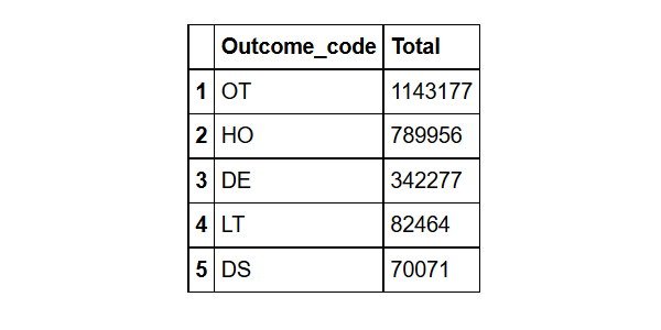
What are the top 5 most common outcomes?
head(outcome,3) # to see the variable names
outcome%>%group_by(Outcome_code= outc_cod)%>% #grouped by Outcome_code
           summarize(Total=n())%>%    # found the count for each Outcome_code
           arrange(desc(Total))%>%    # sorted them in descending order
           head(5)                   # took the top five
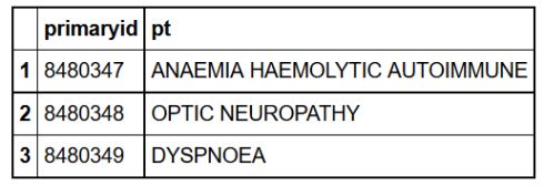
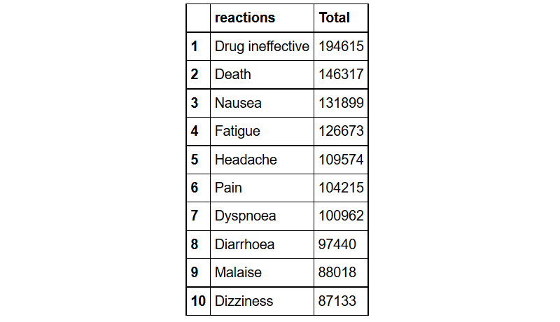
What are the top ten reactions?
head(reaction,3) # to see the variable names
reaction%>%group_by(reactions= pt)%>% # grouped by reactions
           summarize(Total=n())%>%    # found the count for each reaction type
           arrange(desc(Total))%>%    # sorted them in descending order
           head(10)                   # took the top ten
Joins
Let’s join demography, outcome and reaction based on primary id:
inner_joined = demography%>%inner_join(outcome, by='primaryid',copy = TRUE)%>%
               inner_join(reaction, by='primaryid',copy = TRUE)
head(inner_joined)
We can also use primary key and secondary key in our joins. Let’s join drug and indication using two keys (primary and secondary keys).
drug_indication= indication%>%rename(drug_seq=indi_drug_seq)%>%
   inner_join(drug, by=c("primaryid","drug_seq"))
head(drug_indication)
In this post, we saw how to use the dplyr package to create a database and upload data to the database. We also saw how to perform various analytics by querying data from the database.
Working with databases in R has huge advantage when our data is big where loading it to R is impossible or slows down our analytics. If our data resides in a database, rather than loading the whole data to R, we can work with subsets or aggregates of the data that we are interested in. Further, if we have many data files, putting our data in a database, rather than in csv or other format, has better security and is easier to manage.
This is enough for this post. See you in my next post. You can read about dplyr two-table verbs here. If you have any questions or feedback, feel free to leave a comment.


