Through this post I would like to describe a package that I recently developed and published on CRAN. The package titled IMP (Interactive Model Performance) enables interactive performance evaluation & comparison of (binary) classification models.
There are a variety of different techniques available to assess model fit and to evaluate the performance of binary classifiers. As we would expect, there are multiple packages available in R that could be used for this purpose. For instance, the ROCR package is an excellent choice for computing and plotting a range of different performance measures for classification models. The general purpose caret package also provides various options for assessing model fit and evaluating model performance.
While I continue to use these packages, the idea behind trying to create something on my own was triggered by the following considerations:
- Accelerate the model building and evaluation process – Partially automate some of the iterative, manual steps involved in performance evaluation and model fine-tuning by creating small, interactive apps that could be launched as functions (The time saved can then be more effectively utilized elsewhere in the model building process)
- Enable simultaneous comparison of multiple models – Performance evaluation almost always entails comparing the performance of multiple candidate models in an attempt to select a “best” model (basis some definition of what qualifies as “best”). The intent was to write functions that are inherently designed to take multiple model output as arguments, and perform model evaluations simultaneously on them.
- Visualization (using
ggplot2) – Related to the point above; Functions were designed to generate visualizations enabling quick performance comparison of multiple models
Let us now look at some of the key functions from the package and few of the functionalities that it provides:
Analyze Confusion Matrix interactively
Creating a confusion matrix is a common technique to assess the performance of a classification model. The basic idea behind confusion matrix is fairly straightforward – Choose a probability threshold to convert raw probability scores into classes. Comparing the predicted classes with actuals results in 4 possible scenarios (for binary models) which can be represented by a “2 by 2” matrix. This matrix can then be used to compute various measures of performance such as True Positive Rate, False Positive Rate, Precision etc.
(For the purpose of this article, we will assume that you are acquainted with these performance measures. If not, there is a ton of material available online on these topics, which you can read up on)
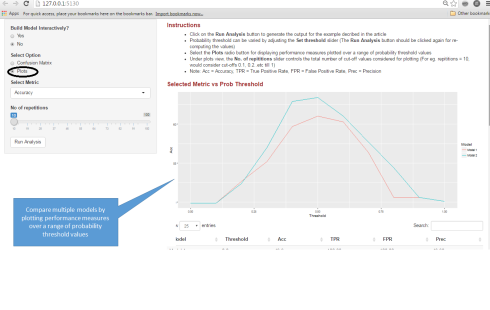
As is obvious, all these measures depend on the probability threshold chosen. Typically, we are interested in computing these measures for a range of different probability values (for e.g. to decide on an optimal cut-off – in situations, where such a cut-off is required) .
Rather than manually invoking a function multiple times (using any one of the many packages that provides an implementation of confusion matrix), it would be easier if we could just invoke a function, which will launch a simple app with probability threshold as a slider input. We could then vary the threshold by adjusting the slider and assess the impact that it has on the confusion matrix and the derived performance measures.
And you could do just that with the interConfMatrix function in the IMP package. Before I provide a demo on how to use this function, let’s broaden the scope of our use case.
Comparing multiple models
As previously highlighted, often times, we have more than one candidate model and we would like to simultaneously evaluate and compare the performance of these models. For e.g. consider we have 2 candidate models and we would like to simultaneously evaluate the impact to confusion matrix (and the derived performance measures) as the probability threshold is varied.
Let us now see how we can use the interConfMatrix function for this:
We will start off by setting up some sample data:
# Let's use the diamonds dataset from the ggplot2 package; Type ?diamonds to read this dataset's documentation
# As an illustrative example, let's try to model the price of the diamond as a function of other attributes
# Price variable is numeric - To convert this into a classification problem lets create a modified variable price_category containing 2 levels - "Above Median"(coded as 1), "Below Median"(coded as 0)

library(ggplot2)

# Lets extract a small subset of the diamonds dataset for our example
diamonds_subset <- diamonds[sample(1:nrow(diamonds), size=1000),]

# Create the price_category variable
diamonds_subset$price_category <- ifelse(diamonds_subset$price > median(diamonds_subset$price),1,0))
Now that we have set up some sample data let’s quickly build 2 simple logistic regression models
# Let's model price as a function of clarity and cut
model_1 <- glm(price_category ~ clarity + cut, data = diamonds_subset, family = binomial())

# Let's update this model by including an additional variable - color
model_2 <- update(model_1, . ~ . + color)

# Now lets use the 'interConfMatrix' function to evaluate confusion matrix for both these models simultaneously
# As you can read from the documentation, this function takes a list of datasets as argument, with each dataframe comprising of 2 columns
# The first column should indicate the class labels (0 or 1) and the second column should provide the raw predicted probabilities

# Lets create these 2 datasets

model1_output <- data.frame(Obs = model_1$y, Pred = fitted(model_1))
model2_output <- data.frame(Obs = model_2$y, Pred = fitted(model_2))

# Lets invoke the interConfMatrix function now - We will put both these dataframes in a list and pass the list as an argument
interConfMatrix(list(model1_output,model2_output))
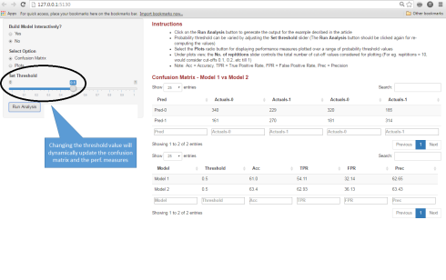
To see a demo of the app that invoking this function will launch, click here. Alternatively, you can view the screenshots from the app attached below:

Updating models interactively
Now let’s increase the interactivity by a notch.
In the previous example, we generated 1 additional candidate model by updating an original model. This is a fairly common procedure as we test out different hypothesis by altering/updating our models (Models can be updated by either dropping some variables, adding new ones, adding interaction effects, non-linear terms etc)
The update function in base R can be used to update an existing model. However, this process can be accelerated if we could do this in an automated & interactive manner.
To do this using the interConfMatrix function we need to do the following: Instead of passing a list of dataframes as an argument, we need to pass 3 different arguments – A model function for generating the model interactively, the dataset name and the y-variable (Dependent Variable) name)
Let us see how:
# The key step here is to define a model function which will take a formula as an argument
# And specify what model should be built and return a dataset as an output
# As before, the dataset should include 2 columns - one for observed values and the other column for predicted raw probability scores

# For the diamonds example described before, we will define a function as follows
glm_model <- function(formula) {
  glm_model <- glm(formula, data = diamonds_subset, family = "binomial")
  out <- data.frame(glm_model$y, fitted(glm_model))
  out }

# Now lets invoke the function - We also need to provide the dataset name and the y variable name
interConfMatrix(model_function = glm_model, data = diamonds_subset, y = "price_category")
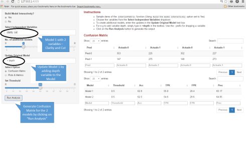
To see a demo of this function, click here. Alternatively, you can view the app screenshot below:

Other model fit & performance measures
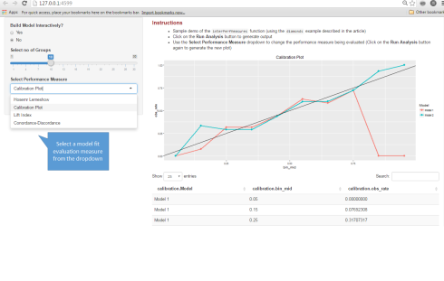
Finally, the package has one other function interPerfMeasures which provides few other model fit and performance evaluation measures. The following tests and performance measures are provided – Hosmer Lemeshow Goodness of Fit test, Concordance-Discordance Measures, Calibration Plots & Lift Index & Gain Charts.
(This function works very similarly to the interConfMatrix described above)
You can see a demo of this function here.
Or, view a screenshot from the app below:

Invoking the functions statically
Both these functions have a static version too – staticConfMatrix and the staticPerfMeasures function. Rather than launch an interactive app, these functions return a list object, when invoked. You can read more about these functions in the package documentation. If you find this useful, do give the package a try!
Hope you found this post useful. If you have any queries or questions, please feel free to comment below or on my github account.
