Working with spatial data is becoming more and more frequent with the development of geoportals providing free access to large number of spatial datasets. Geographic Information System software such as ArcGis or QGis are commonly used to work with these data, in this series of post I want to show the GIS capacities of R.
Spatial data come in two category:
- vector-type: spatial data are represented as discrete elements such as points (cities), lines (rivers) or polygons (countries).
- raster-type: spatial data are represented as regular grids with spatial information discretized into cells / pixels. Raster data are the standard format for remote sensing, satelite data.
In this first post we will see how to work with vector data in R using the sf package.
Getting the data
First we load the needed libraries:
library(tidyverse)
library(sf)
Reading in spatial data into R can be easily done using the st_read function. The function support a large number of formats by using the GDAL driver in the background. We will use an example dataset from the Flemish region of Belgium, downloading a zip file with all the shapefiles, unzipping it and loading it into R:
# define a target directory in your laptop
target_dir <- "./"
# put this as the working directory
setwd(target_dir)
# download the files
download.file("https://downloadagiv.blob.core.windows.net/referentiebestand-gemeenten/VoorlopigRefBestandGemeentegrenzen_2016-01-29/Voorlopig_referentiebestand_gemeentegrenzen_toestand_29_01_2016_GewVLA_Shape.zip", destfile = "municipality.zip")
# unzip it
unzip(zipfile = "municipality.zip")
# read in the Flemish province shapefile
province <- st_read("Shapefile/Refprv.shp")
## Reading layer `Refprv' from data source `D:\Documents\Programming_stuff\lionel68.github.io\_posts_data\r_as_gis\Shapefile\Refprv.shp' using driver `ESRI Shapefile'
## Simple feature collection with 5 features and 8 fields
## geometry type:  MULTIPOLYGON
## dimension:      XY
## bbox:           xmin: 21991.38 ymin: 153049.4 xmax: 258878.5 ymax: 244027.1
## projected CRS:  Belge 1972 / Belgian Lambert 72
The function tells us that te dataset is made of 5 features (rows) each having 8 fields (columns). We also get some infos on the bounding box and the Coordinate Reference System (CRS).
The function returns an object of class sf that looks like a data.frame:
province
## Simple feature collection with 5 features and 8 fields
## geometry type:  MULTIPOLYGON
## dimension:      XY
## bbox:           xmin: 21991.38 ymin: 153049.4 xmax: 258878.5 ymax: 244027.1
## projected CRS:  Belge 1972 / Belgian Lambert 72
##   UIDN OIDN TERRID            NAAM NISCODE NUTS2   LENGTE    OPPERVL
## 1    6    2    357       Antwerpen   10000  BE21 409906.2 2876444170
## 2    7    4    359  Vlaams Brabant   20001  BE24 507999.1 2118893799
## 3    9    5    356 Oost-Vlaanderen   40000  BE23 404985.3 3008166146
## 4   10    1    355         Limburg   70000  BE22 397732.6 2428024237
## 5   11    3    351 West-Vlaanderen   30000  BE25 356653.0 3197075771
##                         geometry
## 1 MULTIPOLYGON (((178133.9 24...
## 2 MULTIPOLYGON (((200484.9 19...
## 3 MULTIPOLYGON (((142473.9 22...
## 4 MULTIPOLYGON (((231635.6 21...
## 5 MULTIPOLYGON (((80189.16 22...
The important difference with a standard data.frame is the “geometry” column that contains the vector informations using the well-known text representation. This column is sticky, it will stay in the R object unless explicitely dropped (check ?st_drop_geometry).
Manipulating sf object
The dplyr functions can be used to manipulate sf objects, for instance we will rename the “NAAM” column, create a new “area” column and sort the rows by the area descending:
province %>%
  rename(name = NAAM) %>%
  mutate(area = OPPERVL / 1e6) %>%
  select(name, area) %>%
  arrange(desc(area)) -> province
Coordinate Reference System
Every spatial data comes with a Coordinate reference system (CRS in short) that describes how the data are represented on the surface of the earth. An in-depth definition of CRS is beyond the scope of this post, here we will just see how to get CRS information from sf object and how to transform them into new reference system.
CRS are defined in sf by their epsg code, for instance the classical GPS/WGS84 CRS has the 4326 code, let's explore this:
# get CRS
st_crs(province)
## Coordinate Reference System:
##   User input: Belge 1972 / Belgian Lambert 72
##   wkt:
## PROJCRS["Belge 1972 / Belgian Lambert 72",
##     BASEGEOGCRS["Belge 1972",
##         DATUM["Reseau National Belge 1972",
##             ELLIPSOID["International 1924",6378388,297,
##                 LENGTHUNIT["metre",1]],
##             ID["EPSG",6313]],
##         PRIMEM["Greenwich",0,
##             ANGLEUNIT["Degree",0.0174532925199433]]],
##     CONVERSION["unnamed",
##         METHOD["Lambert Conic Conformal (2SP)",
##             ID["EPSG",9802]],
##         PARAMETER["Latitude of false origin",90,
##             ANGLEUNIT["Degree",0.0174532925199433],
##             ID["EPSG",8821]],
##         PARAMETER["Longitude of false origin",4.36748666666667,
##             ANGLEUNIT["Degree",0.0174532925199433],
##             ID["EPSG",8822]],
##         PARAMETER["Latitude of 1st standard parallel",49.8333339,
##             ANGLEUNIT["Degree",0.0174532925199433],
##             ID["EPSG",8823]],
##         PARAMETER["Latitude of 2nd standard parallel",51.1666672333333,
##             ANGLEUNIT["Degree",0.0174532925199433],
##             ID["EPSG",8824]],
##         PARAMETER["Easting at false origin",150000.01256,
##             LENGTHUNIT["metre",1],
##             ID["EPSG",8826]],
##         PARAMETER["Northing at false origin",5400088.4378,
##             LENGTHUNIT["metre",1],
##             ID["EPSG",8827]]],
##     CS[Cartesian,2],
##         AXIS["(E)",east,
##             ORDER[1],
##             LENGTHUNIT["metre",1,
##                 ID["EPSG",9001]]],
##         AXIS["(N)",north,
##             ORDER[2],
##             LENGTHUNIT["metre",1,
##                 ID["EPSG",9001]]]]
# re-project into the European CRS
province <- st_transform(province, 3035)
When working with spatial data it is key to make sure that the CRS are adequate, for instance computing areas or distances make more sense in projected CRS rather than in geographic CRS. Also, when doing spatial operations on several spatial objects all the CRS have to be identical.
Plotting spatial data
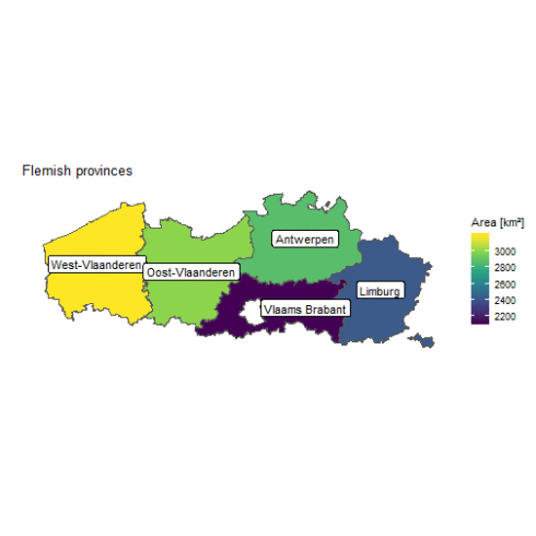
sf objects can be, very convinently, plotted using ggplot2:
# a simple plot of the province
# colored by their surface
ggplot() +
  geom_sf(data = province, aes(fill = area)) +
  geom_sf_label(data = province, aes(label = name)) +
  scale_fill_continuous(type = "viridis",
                        name = "Area [km²]") +
  labs(title = "Flemish provinces",
       x = "",
       y = "") +
  theme(panel.background = element_blank(),
        axis.text = element_blank(),
        axis.ticks = element_blank())
Geometrical operations
Several types of geometrical operations are implemented in sf, we will here explore some of them, you can have a look at this vignette for the full list.
Unary operations returning a geometry
These operations take a single sf object and return geometries, these include getting a buffer around geometries or the centroid of polygons. We will explore this with a dataset of the Flemish municipalities:
# load the municipality shapefile
municipality <- st_read("Shapefile/Refgem.shp")
## Reading layer `Refgem' from data source `D:\Documents\Programming_stuff\lionel68.github.io\_posts_data\r_as_gis\Shapefile\Refgem.shp' using driver `ESRI Shapefile'
## Simple feature collection with 308 features and 9 fields
## geometry type:  MULTIPOLYGON
## dimension:      XY
## bbox:           xmin: 21991.38 ymin: 153049.4 xmax: 258878.5 ymax: 244027.1
## projected CRS:  Belge 1972 / Belgian Lambert 72
# re-project municipality data
municipality <- st_transform(municipality,
                                 st_crs(province))

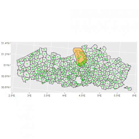
# make a buffer of 5000m around the city of Antwerpen
ant_buffer <- st_buffer(municipality[municipality$NAAM == "Antwerpen",], dist = 5000)

# get the centroids of the municipalities
municipality_cent <- st_centroid(municipality)
## Warning in st_centroid.sf(municipality): st_centroid assumes attributes are
## constant over geometries of x
# plot the different objects
ggplot() +
  geom_sf(data = municipality) +
  geom_sf(data = ant_buffer, alpha = 0.5, fill = "orange") +
  geom_sf(data = municipality_cent, color = "green")
Binary logical operations
These geometrical operation take two geometries and return logical information, for instance we can check which of the city centroids are within the 5km buffer of the city of Antwerpen
st_within(municipality_cent, ant_buffer)
## Sparse geometry binary predicate list of length 308, where the predicate was `within'
## first 10 elements:
##  1: (empty)
##  2: (empty)
##  3: (empty)
##  4: (empty)
##  5: 1
##  6: (empty)
##  7: (empty)
##  8: (empty)
##  9: (empty)
##  10: (empty)
The function returns a list where each element represent the centroid of one of the 308 municipalities, an “(empty)” value means that the centroid was not within the buffer while a value of “1” indicate that it was within the buffer. We can also get this output as a logical vector/matrix:
st_within(municipality_cent, ant_buffer, sparse = FALSE)[1:10,]
##  [1] FALSE FALSE FALSE FALSE  TRUE FALSE FALSE FALSE FALSE FALSE
This can be used to filter the municipality dataset to only keep the cities whose centroid are within the buffer:
municipality %>%
  filter(st_within(municipality_cent, ant_buffer, sparse = FALSE))
## Simple feature collection with 20 features and 9 fields
## geometry type:  MULTIPOLYGON
## dimension:      XY
## bbox:           xmin: 3912907 ymin: 3123760 xmax: 3941971 ymax: 3156259
## projected CRS:  ETRS89-extended / LAEA Europe
## First 10 features:
##    UIDN OIDN TERRID NISCODE       NAAM  DATPUBLBS      NUMAC   LENGTE
## 1   313    5    140   11001 Aartselaar 1982-12-29 1982001920 22122.90
## 2   370   62    124   11029    Mortsel 1982-12-29 1982001920 13450.48
## 3   379   71     85   11040    Schoten 1831-02-07       <NA> 28983.56
## 4   399   91    122   11004   Boechout 1976-01-23 1975123003 26307.31
## 5   400   92    117   11007   Borsbeek 1831-02-07       <NA> 10035.45
## 6   403   95    142   11024    Kontich 1976-01-23 1975123003 29080.36
## 7   418  110     74   11023   Kapellen 1982-07-17 1982001074 29310.94
## 8   482  174     75   11044   Stabroek 1988-09-08 1988000266 21599.21
## 9   490  182    120   46013   Kruibeke 1982-12-29 1982001920 27536.07
## 10  503  195     71   11002  Antwerpen 1988-09-08 1988000266 99479.14
##      OPPERVL                       geometry
## 1   11025465 MULTIPOLYGON (((3929668 313...
## 2    7785306 MULTIPOLYGON (((3933399 313...
## 3   29513750 MULTIPOLYGON (((3941284 314...
## 4   20712116 MULTIPOLYGON (((3938920 313...
## 5    3902970 MULTIPOLYGON (((3935869 313...
## 6   23824644 MULTIPOLYGON (((3930045 313...
## 7   37238543 MULTIPOLYGON (((3932909 315...
## 8   21536451 MULTIPOLYGON (((3929829 315...
## 9   33587947 MULTIPOLYGON (((3924151 313...
## 10 204283071 MULTIPOLYGON (((3926991 315...
All of these operations follow the same logic, st_operation(A, B) checks for each combinations of the geometries in A and B whether A operation B is true or false. For instance st_within(A, B) checks whether the geometries in A are within B, this is similar to st_contains(B, A), the difference between the two being the shape of the returned object. If A has n geometries and B has m, st_contains(B, A) returns a list of length m where each elements contains the row IDs (numbers between 1 and n) of the geometries in A satisfying the operation. By using sparse=FALSE the functions returns matrices, like st_within(A, B, sparse=FALSE) returns a n x m matrix, st_within(B, A, sparse=FALSE) returns a m x n matrix. Note that running st_operation(A, A) checks the operation between all geometries of the object, so returning a n x n matrix.
There are a large number of such operations implemented in sf, you can check ?st_intersects for a list of options. These functions work for any type of geometries (points, lines, polygons), you can check this figure for a graphical representation of some of the operations.
Another example of such binary operations would be to count how many municipalities are within each province:
mat <- st_contains(province, municipality_cent, sparse = FALSE)
province$municipality_count <- apply(mat, 1, sum)
province
## Simple feature collection with 5 features and 3 fields
## geometry type:  MULTIPOLYGON
## dimension:      XY
## bbox:           xmin: 3799513 ymin: 3074638 xmax: 4032508 ymax: 3167919
## projected CRS:  ETRS89-extended / LAEA Europe
##              name     area                       geometry
## 1 West-Vlaanderen 3197.076 MULTIPOLYGON (((3859766 316...
## 2 Oost-Vlaanderen 3008.166 MULTIPOLYGON (((3921616 315...
## 3       Antwerpen 2876.444 MULTIPOLYGON (((3958497 316...
## 4         Limburg 2428.024 MULTIPOLYGON (((4009899 313...
## 5  Vlaams Brabant 2118.894 MULTIPOLYGON (((3976903 311...
##   municipality_count
## 1                 64
## 2                 65
## 3                 69
## 4                 44
## 5                 65
Binary operation returning a geometry
These operations extend the functions seen in the previous section by returning the corresponding geometries, for instance if we want to compute the areas of the intersection of the 5km buffer around Antwerpen with the municipalities:
municipality %>%
  st_intersection(., st_geometry(ant_buffer)) %>%
  mutate(area = st_area(.)) %>%
  mutate(prop_area = as.numeric(area / OPPERVL)) %>%
  arrange(prop_area) -> municipality_inter
## Warning: attribute variables are assumed to be spatially constant
## throughout all geometries
municipality_inter
## Simple feature collection with 29 features and 11 fields
## geometry type:  GEOMETRY
## dimension:      XY
## bbox:           xmin: 3916863 ymin: 3124856 xmax: 3942025 ymax: 3157429
## projected CRS:  ETRS89-extended / LAEA Europe
## First 10 features:
##    UIDN OIDN TERRID NISCODE      NAAM  DATPUBLBS      NUMAC   LENGTE
## 1   352   44    133   12021      Lier 1982-12-29 1982001920 54049.33
## 2   487  179    128   46025     Temse 1982-12-29 1982001920 36505.16
## 3   554  246    154   12007    Bornem 1976-01-23 1975123003 34757.33
## 4   499  191     64   11022 Kalmthout 1982-12-29 1982001920 44002.17
## 5   589  281    146   11025      Lint 1869-06-30       <NA> 13603.12
## 6   358   50    104   11035     Ranst 1982-12-29 1982001920 32714.08
## 7   392   84     88   11039   Schilde 1982-12-29 1982001920 33382.47
## 8   443  135    163   11005      Boom 1831-02-07       <NA> 12224.58
## 9   387   79    155   11037     Rumst 1982-12-29 1982001920 29597.17
## 10  592  284     76   46003   Beveren 1982-12-29 1982001920 63007.70
##      OPPERVL              area  prop_area                       geometry
## 1   49856712    69998.32 [m^2] 0.00140399 POLYGON ((3938357 3130414, ...
## 2   40111036   478231.03 [m^2] 0.01192268 MULTIPOLYGON (((3920096 313...
## 3   46197971   898380.83 [m^2] 0.01944633 POLYGON ((3922951 3128162, ...
## 4   59441394  1430014.45 [m^2] 0.02405755 POLYGON ((3934127 3153756, ...
## 5    5627892   319806.05 [m^2] 0.05682520 POLYGON ((3934665 3129181, ...
## 6   43665536  5457104.05 [m^2] 0.12497509 POLYGON ((3940083 3133253, ...
## 7   36095176  6511826.42 [m^2] 0.18040711 POLYGON ((3942004 3137363, ...
## 8    7199506  1427152.64 [m^2] 0.19822923 POLYGON ((3926726 3125739, ...
## 9   20142693  5249294.65 [m^2] 0.26060541 POLYGON ((3929559 3126868, ...
## 10 153050589 84895066.28 [m^2] 0.55468631 POLYGON ((3921616 3153206, ...
The important difference with these function is that the geometry column returned correspond not to the geometry column of the inputted objects but to the geometry of the operation itself. The different operations available can be found by checking ?st_intersection. An important point to consider is that the attributes (the columns) of the inputted objects are passed to the results of the operation assuming that the attributes values remains constant. For instance, in the example above the column “OPPERVL” represent the area of the municipalities and is passed on the intersections with no changes.
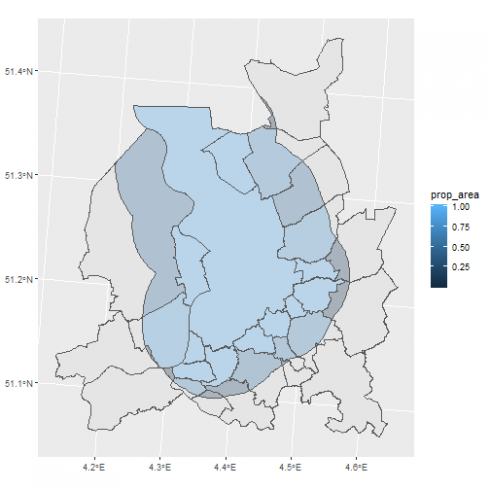
We can check the returned geometries:
ggplot() +
  geom_sf(data = subset(municipality, NAAM %in% municipality_inter$NAAM)) +
  geom_sf(data = municipality_inter, aes(fill = prop_area), alpha = 0.3)
Joins (spatial and non-spatial)
With sf objects different types of joins can be performed, (i) on the attributes (columns) and (ii) on the geometries (spatial).
First we can see joins based on attributes adding population data to the municipality dataset:
# load population file
population <- read.csv("https://raw.githubusercontent.com/lionel68/lionel68.github.io/master/_posts_data/r_as_gis/population_flanders.csv")

# join to the municipality
municipality %>%
  left_join(population) -> municipality_pop
## Joining, by = "NAAM"
For this one can use all the different types of joints available within tidyverse.
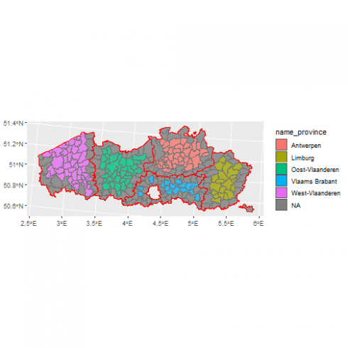
More interesting in this context are spatial joins, for instance joining the province and municipality datasets based on whether the municipalities geometries are within the province geometries:
# slightly adapt names in province
names(province)[1:2] <- paste(names(province)[1:2], "province", sep="_")

# slightly adapt names province
names(municipality_pop)[5] <- "name_municipality"

# joins, using municipality within provinces
municipality_province <- st_join(municipality_pop[,c(5, 10)],
                                 province, join = st_within)

# plot the results
ggplot() +
  geom_sf(data = municipality_province,
          aes(fill = name_province)) +
  geom_sf(data = province, color = "red",
         alpha = 0.2)
We can use for the spatial joins any of the binary logical operations, see ?st_intersects for all the options. These joins are then defined by the join= argument of the function. These joins also works for any types of vector data (point, line, polygon). Here with our examples some of the municipalities were not found to be within any provinces, these were municipalities at the border of the provinces where most likely the borders of the municipalities touched or maybe slightly overflowed out of the provinces.
Use case
To sum up all the things we saw up to know, let's put them in practice by looking at how many inhabitants of Flanders are within 10km of Seveso sites, sites where dangerous (chemical) substances are stored. To do so we will load a dataset containing the geometries of the registered Seveso sites, create buffers, interset this with the municipalities geometries, then assuming that inhabitants are homogeneously distributed over the municipality compute how many inhabitants are in the different intersections.
Let's go:
# load seveso data
seveso <- st_read("https://raw.githubusercontent.com/lionel68/lionel68.github.io/master/_posts_data/r_as_gis/seveso.geojson")
## Reading layer `seveso' from data source `https://raw.githubusercontent.com/lionel68/lionel68.github.io/master/_posts_data/r_as_gis/seveso.geojson' using driver `GeoJSON'
## Simple feature collection with 291 features and 2 fields
## geometry type:  MULTIPOLYGON
## dimension:      XY
## bbox:           xmin: 3809095 ymin: 3082887 xmax: 4012066 ymax: 3164945
## projected CRS:  ETRS89-extended / LAEA Europe
# create 10km buffers
seveso_buffer <- st_buffer(seveso, 10000)
# create intersection with municipality
municipality_seveso <- st_intersection(municipality_pop, seveso_buffer)create 10km buffers
## Warning: attribute variables are assumed to be spatially constant
## throughout all geometries
# compute areas and population within the intersection
# and compute sums
municipality_seveso %>%
  mutate(area_intersection = as.numeric(st_area(.))) %>%
  mutate(pop_intersection = (area_intersection /
                               OPPERVL) * population) %>%
  st_drop_geometry() %>% # we drop the geometry column
  summarise(S_seveso = sum(pop_intersection, na.rm = TRUE),
            S_population = sum(population, na.rm = TRUE)) %>%
  mutate(prop = S_seveso / S_population)
##   S_seveso S_population      prop
## 1 70455290    136289905 0.5169516
Based on the simplified assumptions that municipality population is homogeneously distributed across the municipality area we found that more than half of the inhabitants in Flanders are within 10km of a Seveso site …
Conclusion
In this post the most common GIS operation on vector data were covered using the sf package in R. Make sure to check the very complete Geocomputation in R book for more in-depth infos on this. Next time we will explore raster data, stay tuned!


