I have discovered a new package (at least to me) named Machine Learning Models and Tools for R. The author of this package Brian J Smith describes it as “MachineShop is a meta-package for statistical and machine learning with a unified interface for model fitting, prediction, performance assessment, and presentation of results. Support is provided for predictive modeling of numerical, categorical, and censored time-to-event outcomes and for resample (bootstrap, cross-validation, and split training-test sets) estimation of model performance.” More here.
Using this powerful package I will try to show how it is really much comfortable to create good predictive models with minimal code. Hyperparameter optimization will be also performed by using grid search and random search methods. It is not the scope of this blog post to show why this package works.
So let's start by loading and preparing the dataset in scope. If you're already familiar with data exploration process so you can directly start with the section “Model setup and training”.
Data set and needed packages
Load the needed packages:
devtools::install_github("brian-j-smith/MachineShop", ref = "develop")
## Skipping install of 'MachineShop' from a github remote, the SHA1 (cb60da45) has not changed since last install.
##   Use `force = TRUE` to force installation
The learning problem(as an example) is a binary classification problem. We will be using the credit_data data set available in the {modeldata} package.
Load the data set.
#load dataset
data("credit_data")
# to make the code generic
data_set <- data("credit_data")
data_in_scope <- credit_data%>% plyr::rename(c("Status" = "Target"))
Data Exploration
In this section, some exploratory insights into the data in scope will be given. For exploring the data we will be using the {DataExplorer} package. Introduction to this package can be found here.
Fully conducting EDA and features engineering is not the scope of this blog, but it is highly recommended to have a look at the book from Max Kuhn and Kjell Johnson, which is available here Feature Engineering and Selection: A Practical Approach for Predictive Models, The goal of this book is to help practitioners build better models by focusing on the predictors.
# Get introduced to the dataset:
introduce(data_in_scope)
##   rows columns discrete_columns continuous_columns all_missing_columns total_missing_values complete_rows total_observations memory_usage
## 1 4454      14                5                  9                   0                  455          4039              62356       256216
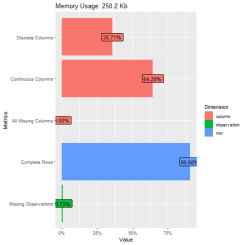
# visualize the table above (with some light analysis):
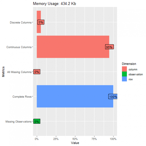
plot_intro(data_in_scope)
Missing values
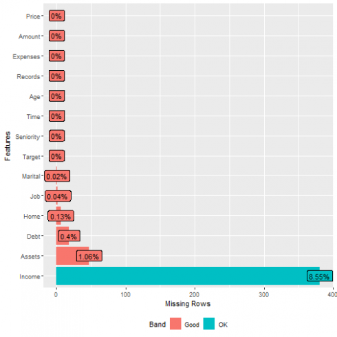
Are there any missing values in our data and which rows have missing values ?
# Missing values ?
plot_missing(data_in_scope)
From the table above we can see that for these data, there were 455 missing values. How we will deal with the missing values is described in section “Missing value treatment”.
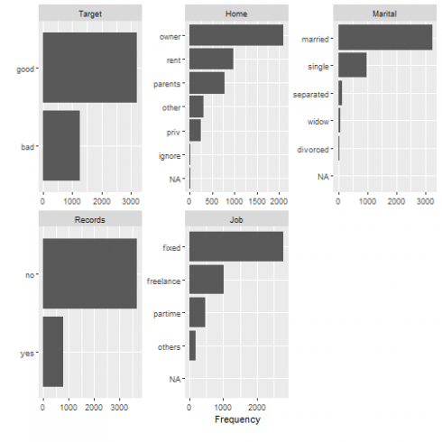
Distributions
#  visualize frequency distributions for all discrete features:
plot_bar(data_in_scope)
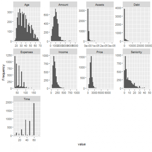
Histograms
# visualize distributions for all continuous features
plot_histogram(data_in_scope)
Target variable analysis
Check severity of class imbalance
# Severity of class imbalance
round(prop.table(table(data_in_scope$Target)), 2)
##
##  bad good
## 0.28 0.72
For the data at hand there is no need to conduct downsampling or upsampling, but if you have to balance your data you can use the function step_downsample() or step_upsample() to reduce the imbalance between majority and minority class.
Correlation analysis
# visualize correlation heatmap for all non-missing features:
plot_correlation(na.omit(data_in_scope))
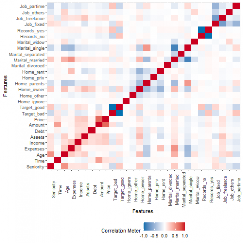
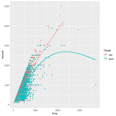
From the plot above we can see for example that the variables Price and Amount are relative high correlated. Just to verify the correlation between the variables “Price” and “Amount, let's visualize the exiting correlation for those variables.
# Visualize the correlation btween "Price" and "Amount"
ggplot2::ggplot(data_in_scope, aes(x = Price, y = Amount, color = Target))+ geom_point() + geom_smooth(se = FALSE)
## `geom_smooth()` using method = 'gam' and formula 'y ~ s(x, bs = "cs")'
We will be using the {recipes} function step_corre() to remove predictors that are highly correlated.
Scatterplots
sample_data <- data_in_scope[ , c("Seniority", "Time", "Age", "Expenses", "Income", "Assets" ,   "Debt" ,     "Amount" ,   "Price")]
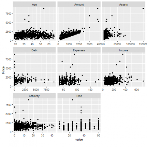
plot_scatterplot(sample_data, by= "Price", sampled_rows = 1000L)
## Warning: Removed 94 rows containing missing values (geom_point).
End data exploration
Preparing the data
Missing value treatment
Usually I use the function set_knnimput()(Imputation via K-Nearest Neighbors) from the {recipes} package to replace the missing values. By training my recipe I first didn't get any failure message, but if I check the trained recipe I got the following message: Training data contained 2969 data points and 299 incomplete rows and this bothers me. So that is the reason why I will use missForest-package {missForest} method, which is a Nonparametric Missing Value Imputation using Random Forest, to replace the missing values.
# Replacing the missing values
set.seed(2020)
imputation_result  <- missForest(data_in_scope, verbose = TRUE )
##   missForest iteration 1 in progress...done!
##     estimated error(s): 0.8435234 0.1398853
##     difference(s): 0.007242625 0.0001347104
##     time: 20.42 seconds
##
##   missForest iteration 2 in progress...done!
##     estimated error(s): 0.8303788 0.1474782
##     difference(s): 0.001674115 0
##     time: 19.86 seconds
##
##   missForest iteration 3 in progress...done!
##     estimated error(s): 0.8284002 0.1480608
##     difference(s): 0.0005001059 0
##     time: 19.85 seconds
##
##   missForest iteration 4 in progress...done!
##     estimated error(s): 0.8469438 0.1459031
##     difference(s): 0.0001399162 0
##     time: 19.72 seconds
##
##   missForest iteration 5 in progress...done!
##     estimated error(s): 0.8375994 0.1446909
##     difference(s): 0.0005071806 0
##     time: 19.85 seconds
data_in_scope_imputed <- imputation_result$ximp

# Check if the data contains missing values
sum(is.na(data_in_scope_imputed))
## [1] 0
Split data into training and testing data
We will split the data into training and testing data. The training data will be used to build the model and the testing data will be used to show how the model is performing on the unseen data (in our case set_for_testing data set).
## Training and test sets
set.seed(2020)
train_indices <- sample(nrow(data_in_scope_imputed), nrow(data_in_scope_imputed) * 2 / 3)
set_for_training <- data_in_scope_imputed[train_indices, ]
set_for_testing <- data_in_scope_imputed[-train_indices, ]
Pre-processing the data using the {recipes} package
We will be using the {recipes} package to pre-process the data and create the design matrix. More information about this concept can be found Here. We create the recipe and assign the steps for preprocessing the data.
#  Pre-Processing the data with{recipes}
set.seed(2020)
rec <- recipe(Target ~., data = set_for_training) %>% # Formula
  role_case(stratum = Target)%>%
  # step_knnimpute(all_predictors(), neighbors = 4)%>%  # Impute missing data
  step_dummy(all_nominal(), -Target) %>%
  step_nzv(all_predictors())%>%                   # remove variables that are highly sparse and unbalanced.
  step_corr(all_predictors()) %>%                 # remove variables that have large absolute correlations with other variables.
  step_center(all_numeric(), -all_outcomes())%>%  # normalize numeric data to have a mean of zero.
  step_scale(all_numeric(), -all_outcomes())      # normalize numeric data to have a standard deviation of one.
Preparing the training and testing data
We will apply the prep function to train the recipe(rec) and prepare the final training and test sets.
# train the data recipe with the function prep
trained_rec <-  prep(rec, training = set_for_training, retain = TRUE)
# Apply the trained recipe to creat the final train set and test set
train_data_cred <- as.data.frame(juice(trained_rec))
test_data_cred  <- as.data.frame( bake(trained_rec, new_data = set_for_testing))
Now let's check if we have really cleaned the data set.
plot_intro(train_data_cred)
We can note that the prepared data is all numeric (but the target variable, which is a factor) with no missing variables.
Model setup and training
Now we're ready to start training the model to the training set, for that we will be using the {MachineShop} package. The available models from the {MachineShop} package can be found via the function modelinfo():
# Show the available models
modelinfo()%>%names()
##  [1] "AdaBagModel"         "AdaBoostModel"       "BARTModel"           "BARTMachineModel"    "BlackBoostModel"     "C50Model"            "CForestModel"
##  [8] "CoxModel"            "CoxStepAICModel"     "EarthModel"          "FDAModel"            "GAMBoostModel"       "GBMModel"            "GLMBoostModel"
## [15] "GLMModel"            "GLMStepAICModel"     "GLMNetModel"         "KNNModel"            "LARSModel"           "LDAModel"            "LMModel"
## [22] "MDAModel"            "NaiveBayesModel"     "NNetModel"           "PDAModel"            "PLSModel"            "POLRModel"           "QDAModel"
## [29] "RandomForestModel"   "RangerModel"         "RPartModel"          "SelectedModel"       "StackedModel"        "SuperModel"          "SurvRegModel"
## [36] "SurvRegStepAICModel" "SVMModel"            "SVMANOVAModel"       "SVMBesselModel"      "SVMLaplaceModel"     "SVMLinearModel"      "SVMPolyModel"
## [43] "SVMRadialModel"      "SVMSplineModel"      "SVMTanhModel"        "TreeModel"           "TunedModel"          "XGBModel"            "XGBDARTModel"
## [50] "XGBLinearModel"      "XGBTreeModel"
For our case study we will be using the RangerModel. To have the default configuration of the selected model we will apply the function modelinfo() on RangerModel.
# Show the default configuration of the selected model(RangerModel)
modelinfo(RangerModel)
## $RangerModel
## $RangerModel$label
## [1] "Fast Random Forests"
##
## $RangerModel$packages
## [1] "ranger"
##
## $RangerModel$response_types
## [1] "factor"  "numeric" "Surv"
##
## $RangerModel$arguments
## function (num.trees = 500, mtry = NULL, importance = c("impurity",
##     "impurity_corrected", "permutation"), min.node.size = NULL,
##     replace = TRUE, sample.fraction = ifelse(replace, 1, 0.632),
##     splitrule = NULL, num.random.splits = 1, alpha = 0.5, minprop = 0.1,
##     split.select.weights = NULL, always.split.variables = NULL,
##     respect.unordered.factors = NULL, scale.permutation.importance = FALSE,
##     verbose = FALSE)
## NULL
##
## $RangerModel$grid
## [1] TRUE
##
## $RangerModel$varimp
## [1] TRUE
Fit default model and Performance
To fit the model to the training set we call the function fit() with the following parameters:
. Unprepared recipe (rec)
. Rangmodel our selected model
# modeling using rec
set.seed(2020)
# Register multiple cores for parallel computations, not strictly necessary, just for speed
registerDoParallel(cores = 4)
# Fit the model
tic()
model_dafault_fit <- fit(rec, model = RangerModel)
toc()
## 0.52 sec elapsed
Show the configuration of the fitted model.
# Show the configuration of the trained model
model_dafault_fit
## Ranger result
##
## Call:
##  ranger::ranger(formula, data = as.data.frame(data), case.weights = weights,      probability = is(response(data), "factor"), ...)
##
## Type:                             Probability estimation
## Number of trees:                  500
## Sample size:                      2969
## Number of independent variables:  18
## Mtry:                             4
## Target node size:                 10
## Variable importance mode:         impurity
## Splitrule:                        gini
## OOB prediction error (Brier s.):  0.1460735
Test set model performance
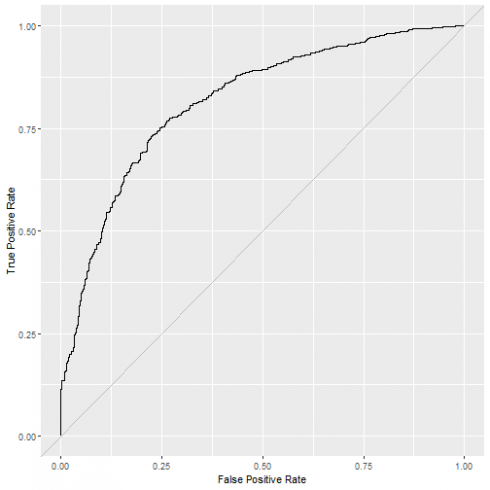
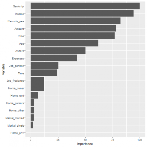
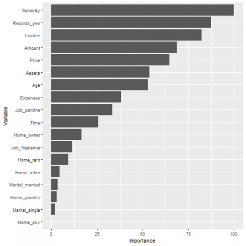
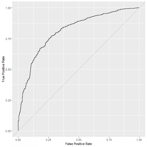
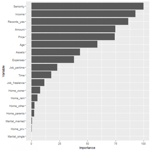
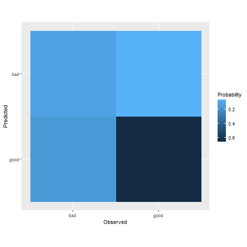
Using the function performance() from the {MachineShop} package we can compute the metrics. But we will define a helper function, which will be used not only to compute the performance but it will also return ROC curve and the confusion matrix and the variable importance. The arguments of this function are the "fitted model” and the “new data” (unseen before).
my_performance_func <- function(model, newData){

  obs <- response(model, newdata = newData)
  pred <- predict(model, newdata = newData, type = "prob")
  perfo <- performance(obs, pred)

 confusion_matrix <- confusion(obs, pred, cutoff = 0.5)
 plot_con <- plot(confusion_matrix)
 curve_plot <- plot(performance_curve(obs, pred), diagonal = TRUE)
 ## Variable importance
vi <- varimp(model)
plt_vip <- plot(vi)

 new_list <- list("Performance, KPIs" = perfo, "ROC Curve" = curve_plot, "Variable Importance"=  plt_vip, "Plot Confusion Matrix " = plot_con)
 return(new_list)
}
Performance of the fitted model
Results: KPIs (Brier, Accuracy, Kappa, ROC AUC , Sensitivity and Specificity), ROC curve, variable importance and the confusion matrix.
Note that we have to use the unprepared test set (set_for_testing) !.
## Test set performance
my_performance_func(model_dafault_fit, set_for_testing)
## $`Performance, KPIs`
##       Brier    Accuracy       Kappa     ROC AUC Sensitivity Specificity
##   0.1480260   0.7824916   0.3798364   0.8167865   0.9264432   0.4063260
##
## $`ROC Curve`
##
## $`Variable Importance`
##
## $`Plot Confusion Matrix `
Do we need to tune the model ? let's see if we can get better performance. Also here tuning the model can be done with minimal code !.
Model tuning using Grid Search method
Grid Search method is an exhaustive search (blind search/unguided search) over a manually specified subset of the hyperparameter space. This method is a computationally expensive option but guaranteed to find the best combination in your specified grid.
With the function TunedModel() we will conduct model tuning over a grid of parameters.
# Ranger model tuned with the training set
set.seed(2020)
# Register multiple cores for parallel computations, not strictly necessary, just for speed
library(doParallel)
registerDoParallel(cores = 4)
tic()
model_fit_tuned <- TunedModel(RangerModel,                # Selected model
                              grid = 10,                  # Number of parameters-specific values to generate outomatically
                              control = CVControl,        # Define the resampling method
                              metrics = "roc_auc")%>%     # Define the metrics
                              fit(rec)                    # Fit the recipe


##

TunedModel(10)
##
1: ModelRecipe | RangerModel

2: ModelRecipe | RangerModel

3: ModelRecipe | RangerModel


4: ModelRecipe | RangerModel


5: ModelRecipe | RangerModel


6: ModelRecipe | RangerModel


7: ModelRecipe | RangerModel


8: ModelRecipe | RangerModel


9: ModelRecipe | RangerModel


10: ModelRecipe | RangerModel
toc()
## 42.89 sec elapsed
# Results of the tuned model/Configuartion
(as.MLModel(model_fit_tuned))
## Object of class "MLModel"
##
## Model name: RangerModel
## Label: Trained Fast Random Forests
## Package: ranger
## Response types: factor, numeric, Surv
## Tuning grid: TRUE
## Variable importance: TRUE
##
## Parameters:
## List of 10
##  $ num.trees                   : num 500
##  $ mtry                        : num 2
##  $ importance                  : chr "impurity"
##  $ replace                     : logi TRUE
##  $ sample.fraction             : num 1
##  $ num.random.splits           : num 1
##  $ alpha                       : num 0.5
##  $ minprop                     : num 0.1
##  $ scale.permutation.importance: logi FALSE
##  $ verbose                     : logi FALSE
##
## TrainStep1 :
## Object of class "TrainBit"
##
## Grid (selected = 1):
## # A tibble: 10 x 1
##    Model$mtry
##         <dbl>
##  1          2
##  2          4
##  3          6
##  4          7
##  5          9
##  6         11
##  7         13
##  8         14
##  9         16
## 10         18
##
## Object of class "Performance"
##
## Metrics: roc_auc
## Models: RangerModel.1, RangerModel.2, RangerModel.3, RangerModel.4, RangerModel.5, RangerModel.6, RangerModel.7, RangerModel.8, RangerModel.9, RangerModel.10
##
## Selected model: RangerModel.1
## roc_auc value: 0.8321219
Performance of the tuned model (Grid Search)
Results: KPIs (Brier, Accuracy, Kappa, ROC AUC , Sensitivity and Specificity), ROC curve and the confusion matrix.
## Test set performance
my_performance_func(model_fit_tuned, set_for_testing)
## $`Performance, KPIs`
##       Brier    Accuracy       Kappa     ROC AUC Sensitivity Specificity
##   0.1498078   0.7764310   0.3237148   0.8206785   0.9534451   0.3138686
##
## $`ROC Curve`

##
## $`Variable Importance`
##
## $`Plot Confusion Matrix `
Voilà we reach better performance, as you can see we did conduct Grid Search (Tune over automatic grid of model parameters) with only one code line. Now let's see if the tuned model over randomly sampled grid points performs better.
Model tuning using Random Search method
Random Search method: a simple alternative and similar to the grid search method but the grid is randomly selected. This method (also blind search/unguided search) is faster at getting reasonable model but will not get the best in your grid.
set.seed(2020)
# Register multiple cores for parallel computations, not strictly necessary, just for speed
library(doParallel)
registerDoParallel(cores = 4)
tic()
model_fit_tuned_randomly <- TunedModel(RangerModel,
                                       grid = Grid(length = 100, random = 10 ),
                                       control = CVControl,
                                       metrics = "roc_auc")%>%
                                       fit(rec)
##

TunedModel(10)
##
1: ModelRecipe | RangerModel


2: ModelRecipe | RangerModel


3: ModelRecipe | RangerModel


4: ModelRecipe | RangerModel


5: ModelRecipe | RangerModel


6: ModelRecipe | RangerModel


7: ModelRecipe | RangerModel


8: ModelRecipe | RangerModel


9: ModelRecipe | RangerModel


10: ModelRecipe | RangerModel
toc()
## 52.76 sec elapsed
(as.MLModel((model_fit_tuned_randomly)))
## Object of class "MLModel"
##
## Model name: RangerModel
## Label: Trained Fast Random Forests
## Package: ranger
## Response types: factor, numeric, Surv
## Tuning grid: TRUE
## Variable importance: TRUE
##
## Parameters:
## List of 12
##  $ num.trees                   : num 500
##  $ mtry                        : num 9
##  $ importance                  : chr "impurity"
##  $ min.node.size               : num 14
##  $ replace                     : logi TRUE
##  $ sample.fraction             : num 1
##  $ splitrule                   : chr "gini"
##  $ num.random.splits           : num 1
##  $ alpha                       : num 0.5
##  $ minprop                     : num 0.1
##  $ scale.permutation.importance: logi FALSE
##  $ verbose                     : logi FALSE
##
## TrainStep1 :
## Object of class "TrainBit"
##
## Grid (selected = 8):
## # A tibble: 10 x 1
##    Model$mtry $min.node.size $splitrule
##         <dbl>          <dbl> <chr>
##  1          2              2 extratrees
##  2         18             16 gini
##  3          5              3 extratrees
##  4         11              2 gini
##  5          7              8 extratrees
##  6         18              4 extratrees
##  7         14             18 extratrees
##  8          9             14 gini
##  9         11             14 extratrees
## 10         17             12 extratrees
##
## Object of class "Performance"
##
## Metrics: roc_auc
## Models: RangerModel.1, RangerModel.2, RangerModel.3, RangerModel.4, RangerModel.5, RangerModel.6, RangerModel.7, RangerModel.8, RangerModel.9, RangerModel.10
##
## Selected model: RangerModel.8
## roc_auc value: 0.8275267
Performance of the tuned model (Random Search)
We call the helper function on the tuned model and the test set.
Results:
KPIs (Brier, Accuracy, Kappa, ROC AUC , Sensitivity and Specificity),
ROC curve,
Variable Importance,
The confusion matrix.
my_performance_func(model_fit_tuned_randomly, set_for_testing)
## $`Performance, KPIs`
##       Brier    Accuracy       Kappa     ROC AUC Sensitivity Specificity
##   0.1489939   0.7804714   0.3882356   0.8133045   0.9124767   0.4355231
##
## $`ROC Curve`
##
## $`Variable Importance`
##
## $`Plot Confusion Matrix `
Performance Summary
The table below is showing the performance of the default model and the performance of the model after conduction of Hyperparameter tuning via Grid Search and Random Search. As we can see the tuned model via Grid Search outperforms.
default <- my_performance_func(model_dafault_fit, set_for_testing)[[1]]
default <- as.data.frame(default)
grid_search <- my_performance_func(model_fit_tuned, set_for_testing)[[1]]
grid_search <- as.data.frame(grid_search)
random_search <- my_performance_func(model_fit_tuned_randomly, set_for_testing)[[1]]
random_search <- as.data.frame(random_search)
all_ <- cbind(default, grid_search, random_search)
print(all_, digits = 3)
##             default grid_search random_search
## Brier         0.148       0.150         0.149
## Accuracy      0.782       0.776         0.780
## Kappa         0.380       0.324         0.388
## ROC AUC       0.817       0.821         0.813
## Sensitivity   0.926       0.953         0.912
## Specificity   0.406       0.314         0.436
Ensembling Strategy
I can not close this article without talking about ensemble learning methods.
From wiki in statistics and machine learning, ensemble methods use multiple learning algorithms to obtain better predictive performance than could be obtained from any of the constituent learning algorithms alone. Unlike a statistical ensemble in statistical mechanics, which is usually infinite, a machine learning ensemble consists of only a concrete finite set of alternative models, but typically allows for much more flexible structure to exist among those alternatives.
In this package two ensembling learning methods are implemented: stacked regression (combine the predictions of several other learning algorithms) and super learners (generalization of stacked regression that fit a specified model). More here
Stacked method
Let's construct an stacked model and see if we will obtain better predictive performance.
The stackedModel consists of the following models:
. XGBModel
. EarthModel
# Stacked regression
stackedmodel <- StackedModel(XGBModel, RangerModel, EarthModel)
res_stacked <- resample(Target ~., data = train_data_cred,  model = stackedmodel)
## ModelFrame | StackedModel
Below are the results of the stacked regression:
summary(res_stacked)
##              Statistic
## Metric             Mean    Median          SD       Min       Max NA
##   Brier       0.1400581 0.1411337 0.008441332 0.1203509 0.1522805  0
##   Accuracy    0.7931941 0.7895429 0.020050432 0.7676768 0.8383838  0
##   Kappa       0.4477924 0.4446214 0.048807639 0.3802030 0.5604070  0
##   ROC AUC     0.8435525 0.8427533 0.021171966 0.8100525 0.8892242  0
##   Sensitivity 0.9078107 0.9105767 0.026219357 0.8591549 0.9483568  0
##   Specificity 0.5041877 0.5029412 0.039373457 0.4166667 0.5595238  0
Super learner method
Now let's construct a superlearner just to show how we can build such a model out of the box !
The constituent learning algorithms are the XGBModel and the EarthModel.
# Model specification
sel_model <- SelectedModel(RangerModel,
  TunedModel(RangerModel),
  SuperModel( XGBModel, TunedModel(EarthModel))
)
Please don't forget to install the selected models for building the Supermodel (in my case xgboost and Earth) !!
# Register multiple cores for parallel computations, not strictly necessary, just for speed
library(doParallel)
registerDoParallel(cores = 4)
# Fit the model
tic()
model_ensemble__fit <- fit(rec, model = sel_model)##
SelectedModel(3)
##
1: ModelRecipe | RangerModel
2: ModelRecipe | TunedModel
3: ModelRecipe | SuperModel

SuperModel(2)
##
1: ModelRecipe | XGBModel
2: ModelRecipe | TunedModel

TunedModel(3)
##
1: ModelRecipe | EarthModel
2: ModelRecipe | EarthModel
3: ModelRecipe | EarthModel
toc()
## 585.44 sec elapsed
as.MLModel(model_ensemble__fit)
## Object of class "SuperModel"
##
## Model name: SuperModel
## Label: Trained Super Learner
## Package:
## Response types: factor, numeric
## Tuning grid: FALSE
## Variable importance: FALSE
##
## Parameters:
## List of 1
##  $ all_vars: logi FALSE
##
## Super learner:
##
## Object of class "MLModelFunction"
##
## Model name: GBMModel
## Label: Generalized Boosted Regression
## Package: gbm
## Response types: factor, numeric, PoissonVariate, Surv
## Tuning grid: TRUE
## Variable importance: TRUE
##
## Arguments:
## function (distribution = NULL, n.trees = 100, interaction.depth = 1,
##     n.minobsinnode = 10, shrinkage = 0.1, bag.fraction = 0.5)
## NULL
##
## Base learners:
##
## Learner1 :
## Object of class "MLModel"
##
## Model name: XGBModel
## Label: Extreme Gradient Boosting
## Package: xgboost
## Response types: factor, numeric, PoissonVariate
## Tuning grid: FALSE
## Variable importance: TRUE
##
## Parameters:
## List of 4
##  $ params       : list()
##  $ nrounds      : num 1
##  $ verbose      : num 0
##  $ print_every_n: num 1
##
## Learner2 :
## Object of class "TunedModel"
##
## Model name: TunedModel
## Label: Grid Tuned Model
## Package:
## Response types: factor, numeric
## Tuning grid: FALSE
## Variable importance: FALSE
##
## Tuning parameters:
##
## Object of class "MLModelFunction"
##
## Model name: EarthModel
## Label: Multivariate Adaptive Regression Splines
## Package: earth
## Response types: factor, numeric
## Tuning grid: TRUE
## Variable importance: TRUE
##
## Arguments:
## function (pmethod = c("backward", "none", "exhaustive", "forward",
##     "seqrep", "cv"), trace = 0, degree = 1, nprune = NULL, nfold = 0,
##     ncross = 1, stratify = TRUE)
## NULL
##
## Object of class "Grid"
##
## Length: 3
## Random sample: FALSE
##
## Object of class "MLControl"
##
## Name: CVControl
## Label: K-Fold Cross-Validation
## Folds: 10
## Repeats: 1
## Seed: 1674321957
##
## Object of class "MLControl"
##
## Name: CVControl
## Label: K-Fold Cross-Validation
## Folds: 10
## Repeats: 1
## Seed: 1185010321
##
## TrainStep1 :
## Object of class "TrainBit"
##
## Grid (selected = 3):
## # A tibble: 3 x 1
##   Model
##   <fct>
## 1 1
## 2 2
## 3 3
##
## Object of class "Performance"
##
## Metrics: Brier, Accuracy, Kappa, ROC AUC, Sensitivity, Specificity
## Models: RangerModel, TunedModel, SuperModel
##
## Selected model: SuperModel
## Brier value: 0.1432923
# Compute the performance of the superlearner model
obs_r <- response(model_ensemble__fit, newdata = set_for_testing )
pred_r <- predict(model_ensemble__fit, newdata = set_for_testing, type = "prob")
performance(obs_r, pred_r)
##       Brier    Accuracy       Kappa     ROC AUC Sensitivity Specificity
##   0.1456026   0.7858586   0.4072213   0.8220095   0.9124767   0.4549878
Conclusion and Outlook
I hope this end-to-end example could illustrate how you can use this powerful package {MachineShop} to conduct predictive modeling and tuning the Hyperparameter in a relative easy and well structured way.
At this point of time the Bayesian Hyperparameter Tuning method is not implemented in this package. I hope this method will be implemented in the near future.
I hope the time will allow me to finalize the Shiny app, which we can use to fit other MachineShop models and conducting Hyperparameter tuning with only a few clicks.
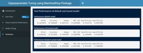
The following picture is giving an example of what we can produce with this Shiny app:
If you're interested on the first version of this Shiny app and/or you would like to contribute to develop an optimal Shiny app so let me know at kritiker2017@gmail.com I will be happy to share with you the source code.
I would like to thank;
Brian J Smith the developer of the {MachineShop} package,
Max Kuhn and Kjell Johnson the developers of the {recipes} package,
Boxuan Cui the developer of the {DataExplorer} package,
and all the developers of packages I have used in this blog post.
