Survey data remains an integral part of organizational science and rightfully so. With ever-increasing means of data collection brought about by more nuanced and faster technologies, organizations have no shortage of data – but it would be remiss to discount the value of self-report data to better understand the psychology of workers. Alas, not all surveys are created equal, or rather equally well; so, it’s important to utilize scientifically established methods to evaluate them and draw the appropriate inferences from the data collected.
The full survey construction process should include the following:
1. Define the construct and content domain (e.g., emotional intelligence.)
2. Generate items to cover the content domain
3. Assess content validity
4. Large scale administration
5. Exploratory factor analysis
6. Internal consistency reliability analysis (i.e., Cronbach’s alpha)
7. Confirmatory factor analysis
8. Convergent/discriminant validity evidence
9. Criterion validity evidence
10. Replicate steps 6 – 9 in a new sample(s)
In this article, steps 5 and 6 of the survey evaluation process are covered using R. Another post may potentially address later steps (7-9) so be sure to bookmark this page! For insights or recommendations from your friendly neighborhood I-O psychologist regarding the early stages of survey construction, feel free to contact the author. The construct of interest for this scale development project is human-machine preferences.
Load necessary libraries.
#load libraries
library(tidyverse) #masks stats::filter, lag
library(tibble)
library(psych) #masks ggpplot2:: %+%, alpha
library(GGally) #masks dbplyr::nasa
library(kableExtra) #masks dplyr::group_rows
library(MVN)
Import Data
This survey was developed at a research institution and the IRB protocols mandated that the data are not publicly hosted. A completely de-identified version was used for this walkthrough and preprocessed fully before being analyzed, so a glimpse into the data is provided (pun intended).
Note: Some of the survey items were labeled with “_R” signaling that they are reverse coded. This was handled accordingly in the data preprocessing stage as well.
glimpse(dat)
Rows: 381
Columns: 16
$ HUM1     3, 4, 1, 4, 3, 4…
$ HUM2_R   3, 2, 2, 4, 4, 4…
$ HUM3_R   2, 5, 3, 3, 2, 3…
$ HUM4     2, 3, 3, 2, 3, 3…
$ HUM5     2, 4, 5, 4, 2, 3…
$ HUM6_R   2, 2, 1, 2, 2, 3…
$ HUM7_R   2, 4, 2, 3, 4, 5…
$ HUM8_R   1, 3, 1, 2, 2, 2…
$ HUM9_R   4, 2, 3, 4, 3, 3…
$ HUM10    2, 2, 2, 4, 2, 3…
$ HUM11_R  3, 2, 2, 4, 4, 3…
$ HUM12    4, 4, 4, 4, 3, 5…
$ HUM13_R  1, 4, 1, 2, 2, 3…
$ HUM14_R  3, 4, 2, 4, 3, 3…
$ HUM15_R  2, 4, 1, 4, 3, 2…
$ HUM16_R  2, 5, 2, 2, 2, 3…
summary(dat)
      HUM1           HUM2_R          HUM3_R           HUM4            HUM5
 Min.   :1.000   Min.   :1.000   Min.   :1.000   Min.   :1.000   Min.   :1.000
 1st Qu.:2.000   1st Qu.:2.000   1st Qu.:2.000   1st Qu.:3.000   1st Qu.:3.000
 Median :3.000   Median :3.000   Median :3.000   Median :3.000   Median :4.000
 Mean   :2.869   Mean   :3.055   Mean   :2.832   Mean   :3.105   Mean   :3.714
 3rd Qu.:4.000   3rd Qu.:4.000   3rd Qu.:4.000   3rd Qu.:4.000   3rd Qu.:5.000
 Max.   :5.000   Max.   :5.000   Max.   :5.000   Max.   :5.000   Max.   :5.000
     HUM6_R          HUM7_R          HUM8_R          HUM9_R          HUM10
 Min.   :1.000   Min.   :1.000   Min.   :1.000   Min.   :1.000   Min.   :1.000
 1st Qu.:2.000   1st Qu.:2.000   1st Qu.:1.000   1st Qu.:2.000   1st Qu.:3.000
 Median :2.000   Median :3.000   Median :2.000   Median :3.000   Median :3.000
 Mean   :2.136   Mean   :2.911   Mean   :1.848   Mean   :2.942   Mean   :3.089
 3rd Qu.:3.000   3rd Qu.:4.000   3rd Qu.:2.000   3rd Qu.:4.000   3rd Qu.:4.000
 Max.   :5.000   Max.   :5.000   Max.   :5.000   Max.   :5.000   Max.   :5.000
    HUM11_R          HUM12          HUM13_R         HUM14_R         HUM15_R
 Min.   :1.000   Min.   :1.000   Min.   :1.000   Min.   :1.000   Min.   :1.000
 1st Qu.:3.000   1st Qu.:4.000   1st Qu.:2.000   1st Qu.:3.000   1st Qu.:2.000
 Median :4.000   Median :4.000   Median :2.000   Median :3.000   Median :3.000
 Mean   :3.535   Mean   :4.108   Mean   :2.491   Mean   :3.357   Mean   :3.234
 3rd Qu.:4.000   3rd Qu.:5.000   3rd Qu.:3.000   3rd Qu.:4.000   3rd Qu.:4.000
 Max.   :5.000   Max.   :5.000   Max.   :5.000   Max.   :5.000   Max.   :5.000
    HUM16_R
 Min.   :1.000
 1st Qu.:2.000
 Median :3.000
 Mean   :3.045
 3rd Qu.:4.000
 Max.   :5.000
Exploratory Data Analysis
Pairs Plot
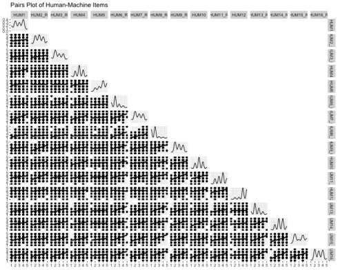
The `GGally` package is an extension of the ubiquitous `ggplot2` visualization library and is incredibly poweful. The ggpairs function creates a pairs plot of the survey items.
(pairsPlot = GGally::ggpairs(data = dat,
                    upper = "blank",
                    diag = list(continuous = wrap("densityDiag")),
                    lower = list(continuous = wrap(ggally_smooth_lm)),
                    title = "Pairs Plot of Human-Machine Items"))
Correlations
Correlation analyses seek to measure the statistical relationship between two (random) variables. There is a range of techniques used to assess the relationship between varying data types with the most well-known being Pearson’s-product moment correlation. This (parametric) analysis is effective when continuous variables have a linear relationship and follow a normal distribution; however, surveys usually include Likert-type response options (e.g., Strongly agree to Strongly disagree) and modeling the data as ordinal can sometimes lead to more accurate parameter estimates…to an extent – as the number of response options increase, the more likely the data can be modeled as continuous anyway because the impact becomes negligible.
Opinions will vary but my personal threshold for the number of response options before modeling the data as continuous is 6, but best practice is probably to model the data a couple of ways in order to establish the best analysis. Check out this article to learn more data types and modeling distributions.
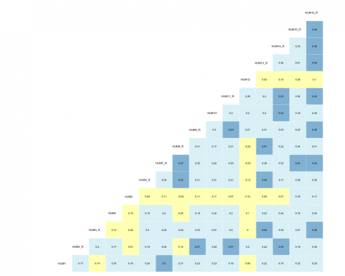
All of the survey items within the current scale utilized a 5-point Likert-type response format and polychoric correlations were calculated. Polychoric correlations help allay the attenuation that occurs when modeling discretized data by using the more appropriate joint distribution. R’s psych library has the polychoric function along with a plethora of others that are particularly useful for survey analysis.
corrs = psych::polychoric(dat)

#correlation viz
GGally::ggcorr(data = NULL,
       cor_matrix = corrs[["rho"]],
       size = 2,
       hjust = .75,
       nbreaks = 7,
       palette = "RdYlBu",
       label = TRUE,
       label_color = "black",
       digits = 2,
       #label_alpha = .3,
       label_round = 2,
       label_size = 1.85,
       layout.exp = 0.2) +
  theme(legend.position = "none")
Parallel Analysis
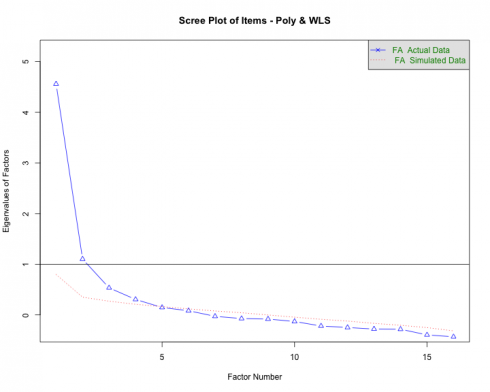
Parallel analysis (PA) is a procedure that helps determine the number of factors (EFA) or components (PCA) to extract when employing dimension reduction techniques. The program is based on the Monte Carlo simulation and generates a data set of random numbers with the same sample size and variables/features as the original data. A correlation matrix of the random data is computed and decomposed thus creating corresponding eigenvalues for each factor — when the eigenvalues from the random data are larger than the eigenvalues from the factor analysis, one has evidence supporting that the factor mostly comprised of random noise.
The current data was subjected to the PA and the following scree plot was produced.
The PA proposes that 3-5 factors most effectively explain the underlying structure of the data. This method is better than some of the older guidelines associated with dimensionality reduction such as the Kaiser criterion that was geared more toward PCA.
Note. PA is an iterative process that needs parameter specifications very similar to EFA (i.e., specified correlation, rotation, estimation method, etc.) and some researchers may conduct the analysis after running the EFAs. Irrespective of the order of operations, the outputs should inform one another.
Exploratory Factor Analysis
Exploratory factor analysis (EFA) is a multivariate approach whose overarching goal is to identify the underlying relationships between measured variables. As briefly mentioned in the PA section, it is entirely based on correlations (the model can account for uncorrelated factors via rotation methods) and is largely used in scale development across disciplines. EFA is but one part of the factor analytic family and a deep dive into the procedure is beyond the scope of this post. Check out UCLA’s link for a practical introduction into the analysis.
An important step in EFA is specifying the number of factors for the model. For this walk-through, the psych package’s fa function was used in a loop to run a series of iterative models between 1 and 5 factors. In psychological research, most of the phenomena investigated are related to one another to some extent, and EFA helps parse out groups that are highly related (within-group) but distinct (between-group) from one another. The model specifies the weighted least squares (WLS) estimation method in an effort to obtain more accurate parameter estimates when using polychoric correlations. Ultimately, five models are individually run and stored in a list so the output(s) can be called and compared.
efa_mods_fun = function(r, n_models = NULL, ...){

    if (!is.matrix(r))
        stop("r must be a matrix of covariances!")

    efa_models = list()

    for (i in seq(n_models)){
        efa_models[[i]] = fa(r,
                             n.obs = nrow(dat),
                             nfactors = i,
                             rotate = "oblimin",
                             # n.iter = 1000,
                             fm = "wls",
                             max.iter = 5000)
    }
    return(efa_models)
}

#run series of models; 1:5-factor solutions
modsEFA_rnd1 = efa_mods_fun(corrs[["rho"]], n_models = 5)
Fit Indices
Note! The code used to extract the fit statistics for each model was not very programmatic, so I redacted it from this tutorial page. Instead, check out the source code in the GitHub repo found here and begin reviewing at line 158. My plan is to eventually develop code that can take a model’s output and generate a table that has the same structure but without the manual repetitiveness. Since this table needs to be created for each iteration of model comparisons, I want to ultimately prevent the likelihood of introducing errors.
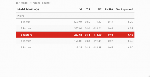
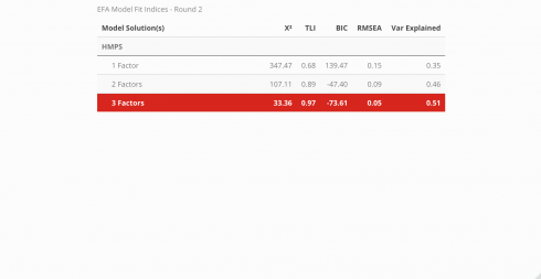
The fit for each model can be compared across a variety of indices. Below, the Chi-squared statistic, Tucker-Lewis Index (TLI), Bayesian Information Criteria (BIC), root mean squared error (RMSEA), and the amount of variance explained by the model are all assessed to determine which model best described the data and is displayed in a neat table using the kableExtra package. To learn more about what the indices measure and what information they convey, visit this link.
#visualize table
modsFit_rnd1 %>%
  rownames_to_column() %>%
  rename(
    'Model Solution(s)' = rowname,
    'X\u00B2' = a,
    'TLI' = b,
    'BIC' = c,
    'RMSEA' = d,
    'Var Explained' = e
  ) %>%
  mutate(
    'Model Solution(s)' = c('1 Factor', '2 Factors', '3 Factors',
                            '4 Factors', '5 Factors')
  ) %>%
  kableExtra::kable('html',
        booktabs = TRUE,
        caption = 'EFA Model Fit Indices - Round 1') %>%
  kable_styling(bootstrap_options = c('striped', 'HOLD_position'),
                full_width = FALSE,
                position = 'center') %>%
  column_spec(1, width = '8cm') %>%
  pack_rows(
    index = c('HMPS ' = 5),
    latex_gap_space = '.70em') %>%
  row_spec(3, bold = T, color = "white", background = "#D7261E")
According to the fit statistics, the 3-factor model best describes the data but the journey does not conclude here because assessing the item level statistics helps determine the structure of the model. Ideally, simple structure is the goal — this means that each item will individually load unto a single factor. When an item loads unto multiple factors it is known as cross-loading. There is nothing inherently “wrong” with cross-loading but for survey development, establishing strict rules provides more benefits in the long run. The cut-off value for a “useful” item loading was set at .45, thus any item that had a loading less than the cut-off was removed before the model was re-run.
Note. Because of the estimation method used in EFA, a factor loading for EACH item and FACTOR will be calculated. The closer the loading value is to 1 the better.
Factor Loading Diagram
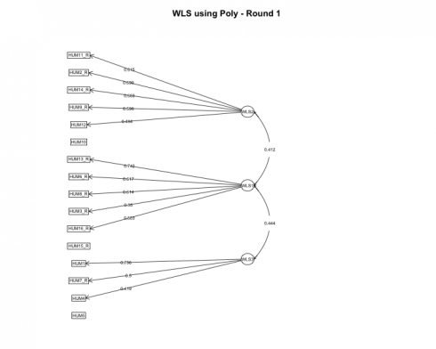
psych::fa.diagram(modsEFA_rnd1[[3]],
           main = "WLS using Poly - Round 1",
           digits = 3,
           rsize = .6,
           esize = 3,
           size = 5,
           cex = .6,
           l.cex = .2,
           cut = .4,
           marg = (c(.5, 2.5, 3, .5)))
Based on our model, each item cleanly loaded unto a single factor and the only item with a loading less than the specified cut-off value was HUM5. It was removed before estimating the models a second time.
Round 2
Most psychometricians recommend removing one item at a time before rerunning the models and calculating fit statistics and item loadings. Unfortunately, I have not developed a streamlined process for this using R (nor has anyone from my very specific Google searches) but perhaps this will be my future contribution to the open source community!
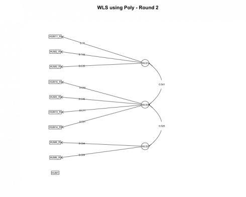
After rerunning the models, again the 3-factor solution is optimal. Let’s review the item loadings next to see how the loadings altered.
The fa.diagram function provides a good overall view of individual item loadings, but the true beauty of R, although a functional programming language, is its ability to operate from an object-oriented paradigm as well. Each model that was run had its respective output so next, let’s extract the loadings from each model and visualize the loadings using ggplot.
#factor loadings of each model
modsEFA_loadings = list()
#loop
for (i in seq_along(modsEFA_rnd2)) {
  modsEFA_loadings[[i]] = rownames_to_column(
    round(data.frame(
      modsEFA_rnd2[[i]][["loadings"]][]), 3),
    var = "Item") %>%
    gather(key = "Factor", value = "Loading", -1)
}
Best Competing Model
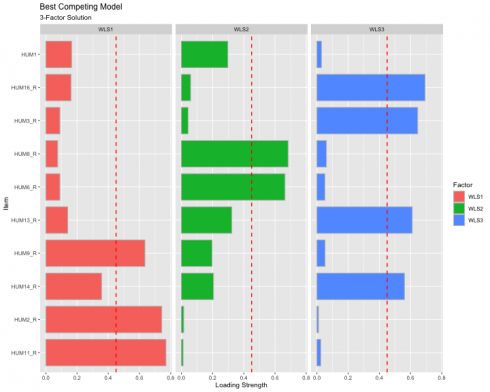
Visualize the individual item loadings from the best competing model: 3-Factor solution!
#viz of factor loadings
ggplot(data = modsEFA_loadings[[3]],
       aes(fct_inorder(Item),
           abs(Loading),
           fill = Factor)
       ) +
  geom_bar(stat = "identity", width = .8, color = "gray") +
  coord_flip() +
  facet_wrap(~ Factor) +
  #scale_x_discrete(limits = rev(unique(loadings[[1]]))) +
    labs(
      title = "Best Competing Model",
      subtitle = "3-Factor Solution",
      x = "Item",
      y = "Loading Strength"
      ) +
    theme_gray(base_size = 10) +
    theme(legend.position = "right") +
  geom_hline(yintercept = .45, linetype = "dashed", color = "red", size = .65)
The red dashed line represents the cut-off value of .45, indicating that anything below the read line is “meaningless” and anything above as “useful.” This visualization also shows the extent to which the items load unto all the factors to help inspect potential cross-loading. We have achieved simple structure since no items are cross-loading.
Conclusion
Hopefully, this tutorial proves to be insightful for survey analysis. The steps included are by no means perfect and the processes will almost certainly change based on the researchers’ choices (e.g., modeling Pearson correlations vs polychoric, setting a more strict factor loading cut-off value, etc.). Regardless of the analytical decisions, using survey science to explore and analyze the development process is vital (and fun!). All code is hosted on GitHub.
