3D Plots built in the right way for the right purpose are always stunning. In this article, we’ll see how to make stunning 3D plots with R using ggplot2 and rayshader . While ggplot2 might be familiar to anyone in Data science, rayshader may not. So, let’s start with a small introduction to rayshader .
Package Description:
rayshader is an open source package for producing 2D and 3D data visualizations in R. rayshader uses elevation data in a base R matrix and a combination of raytracing, spherical texture mapping, overlays, and ambient occlusion to generate beautiful topographic 2D and 3D maps. In addition to maps, rayshader also allows the user to translate ggplot2 objects into beautiful 3D data visualizations.
Required Libraries/Packages:
The latest version of rayshader is available on github which could be installed using either devtools or remotes .
devtools::install_github("tylermorganwall/rayshader")
And, make sure you’ve got the most recent version of ggplot2 . If you are a tidyverse-person, then get the latest of it.
install.packages('tidyverse')
Data
To keep the requirements of this article minimal, We’ll use faithfuld one of the inbuilt datasets in ggplot2 library.
glimpse(faithfuld)
Observations: 5,625
Variables: 3
$ eruptions  1.600000, 1.647297, 1.694595, 1.741…
$ waiting    43, 43, 43, 43, 43, 43, 43, 43, 43,…
$ density    0.003216159, 0.003835375, 0.0044355…
As you can see, faithfuld has got 3 continuous variables which we’ll use for plotting.
2D Plot
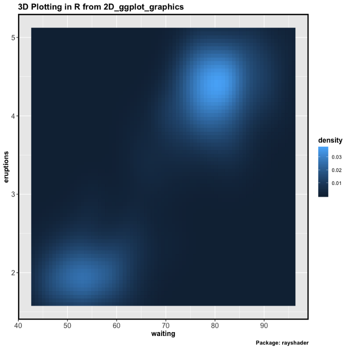
Our journey of a 3D plot just begins with a normal 2D ggplot2 plot. We’ll build a density plot using geom_raster between waiting, eruptions to see how how the data is.
faithful_dd = ggplot(faithfuld, aes(waiting, eruptions)) +
  geom_raster(aes(fill = density)) +
  ggtitle("3D Plotting in R from 2D_ggplot_graphics") +
  labs(caption = "Package: rayshader") +
  theme(axis.text = element_text(size = 12),
        title = element_text(size = 12,face="bold"),
        panel.border= element_rect(size=2,color="black",fill=NA));

faithful_dd
Gives this plot:
Journey from 2D Plot to 3D Plot — One Line!
The journey from a 2D plot to a 3D Plot, is just one extra line of code that comes from the package rayshader . The function plot_gg() which takes a bunch of arguments to define how the 3D plot should look like.
plot_gg(faithful_dd, multicore = TRUE, width = 8, height = 8, scale = 300, zoom = 0.6, phi = 60, background = "#afceff",shadowcolor = "#3a4f70")
faithful_dd is the ggplot2 object that we generated in the previous step. As most of the arguments are self-explanatory like — multicore to activate all the cores of the computer while rendering. Arguments like zoom and phi are to set where the 3D camera view should be.
Imagine, you get to explain Gradient descent or some optimization algorithm like this which is more intuitive and self-explanatory to get a mental model.
This doesn’t end with just a 3D Plot but the developer (Tyler Morgan-Wall) was kind enough to give us another function render_movie() that places a Camera and revolves it around the 3D plot that we just built and gives us a stunning video of the 3D Plot. render_movie() internally uses av package to make a video.
render_movie("faithful_3d.mp4", frames = 480)
Summary
Thanks to Tyler, now we can make stunning 3D Plots from 2D ggplots — just using one extra function plot_gg() ultimately even making a 360-degree video of the 3D Plot. Learn more about Data Visualization in R here and rayshader documentation. The code used and the sessionInfo is available here.

