Image recognition and classification is a rapidly growing field in the area of machine learning. In particular, object recognition is a key feature of image classification, and the commercial implications of this are vast.
For instance, image classifiers will increasingly be used to:
- Replace passwords with facial recognition
- Allow autonomous vehicles to detect obstructions
- Identify geographical features from satellite imagery
These are just a few of many examples of how image classification will ultimately shape the future of the world we live in.
So, let’s take a look at an example of how we can build our own image classifier.
Model Training with VGG16
VGG16 is a built-in neural network in Keras that is pre-trained for image recognition.
Technically, it is possible to gather training and test data independently to build the classifier. However, this would necessitate at least 1,000 images, with 10,000 or greater being preferable.
In this regard, it is much easier to use a pre-trained neural network that has already been designed for image classification purposes.
Purpose of model
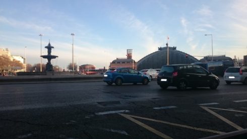
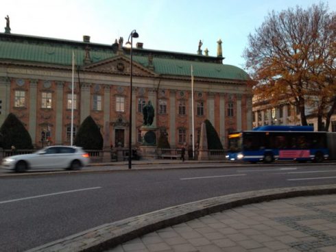
The following are two images of traffic in Madrid, Spain, and Stockholm, Sweden:
The purpose of building an image classifier in this instance is to correctly identify the presence of a vehicle in the image.
As an example, autonomous cars need to have the ability to detect the presence of traffic in real-time in order to avoid a collision. Image recognition (or instantaneously examining each frame in a video for the presence of an object) is how this would be accomplished.
Let’s start with the image of traffic in Madrid city centre.
Classification
Firstly, the libraries are imported and the predictions are generated.
# Import Libraries
from keras.preprocessing.image import load_img
from keras.preprocessing.image import img_to_array
from keras.applications.vgg16 import preprocess_input
from keras.applications.vgg16 import decode_predictions
from keras.applications.vgg16 import VGG16
from keras import backend as K
import matplotlib.pyplot as plt
import numpy as np

# Process Model
model = VGG16()
image = load_img('madrid.jpg', target_size=(224, 224))
image = img_to_array(image)
image = image.reshape((1, image.shape[0], image.shape[1], image.shape[2]))
image = preprocess_input(image)

# Generate predictions
pred = model.predict(image)
print('Predicted:', decode_predictions(pred, top=3)[0])
np.argmax(pred[0])
Here are the generated predictions:
print('Predicted:', decode_predictions(pred, top=3)[0])
Predicted: [('n03788195', 'mosque', 0.578081), ('n03220513', 'dome', 0.16524781), ('n03837869', 'obelisk', 0.08766182)]
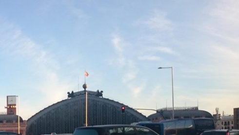
We see that for this instance, the classifier did not do a particularly good job. It did not identify the presence of cars in the image and incorrectly identified the train station as a mosque.
Heatmap
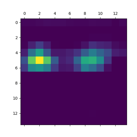
To diagnose this further, it is helpful to use what is called a heatmap. This allows us to determine where precisely the neural network is “zooming in” on the image to make a classification.
Firstly, a Grad-CAM algorithm can be used to generate the heatmap:
# Grad-CAM algorithm
specoutput=model.output[:, 668]
last_conv_layer = model.get_layer('block5_conv3')
grads = K.gradients(specoutput, last_conv_layer.output)[0]
pooled_grads = K.mean(grads, axis=(0, 1, 2))
iterate = K.function([model.input], [pooled_grads, last_conv_layer.output[0]])
pooled_grads_value, conv_layer_output_value = iterate([image])
for i in range(512):
    conv_layer_output_value[:, :, i] *= pooled_grads_value[i]

heatmap=np.mean(conv_layer_output_value, axis=-1)

# Heatmap post processing
heatmap = np.maximum(heatmap, 0)
heatmap /= np.max(heatmap)
plt.matshow(heatmap)
plt.show()
Now, the heatmap is superimposed. In other words, we can view where the zones in the heatmap occur and where the classification is being centered.
# Superimposing heatmap
import cv2
img = cv2.imread('croppedstockholm4.jpg')
heatmap = cv2.resize(heatmap, (img.shape[1], img.shape[0]))
heatmap = np.uint8(255 * heatmap)
heatmap = cv2.applyColorMap(heatmap, cv2.COLORMAP_JET)
superimposed_img = heatmap * 0.4 + img
cv2.imwrite('heatmap4.jpg', superimposed_img)
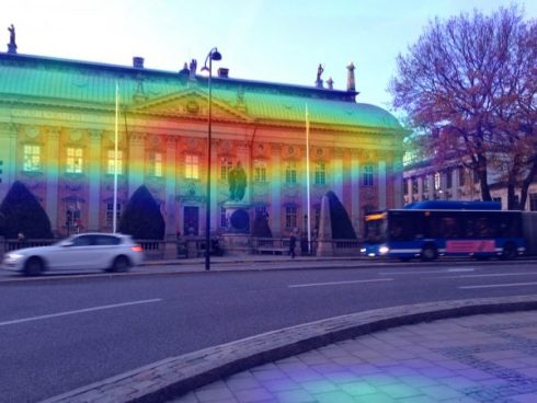
Here is the superimposed image:
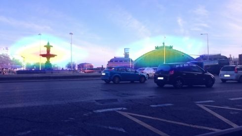
We can see that the heatmap is not focused on the cars in the image. Rather, the focus is on the large building and the water fountain as indicated by the zones in the image.
Cropping images with PIL
However, one way to alleviate this is by cropping the image into four separate quadrants using the PIL library.
The reason for this is that by considering certain areas of the image in isolation, the probability is increased that the image classifier will detect the presence of cars in the image as a whole.
To do this, a base height is set for the image which will be resized, and then the image is cropped into four equal quadrants.
from PIL import Image
baseheight = 700
img = Image.open('madrid.jpg')
hpercent = (baseheight / float(img.size[1]))
width = int((float(img.size[0]) * float(hpercent)))
img = img.resize((width, baseheight), Image.ANTIALIAS)
img.save('resizedimagemadrid.jpg')

h1=baseheight/2
w1=width/2

croppedIm = img.crop((0, 0, w1, h1)) # left, up, right, bottom
croppedIm.save('croppedmadrid1.jpg')

croppedIm = img.crop((0, h1, w1, baseheight)) # left, up, right, bottom
croppedIm.save('croppedmadrid2.jpg')

croppedIm = img.crop((w1, 0, width, h1)) # left, up, right, bottom
croppedIm.save('croppedmadrid3.jpg')

croppedIm = img.crop((w1, h1, width, baseheight)) # left, up, right, bottom
croppedIm.save('croppedmadrid4.jpg')
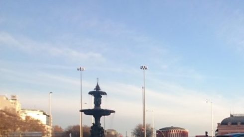
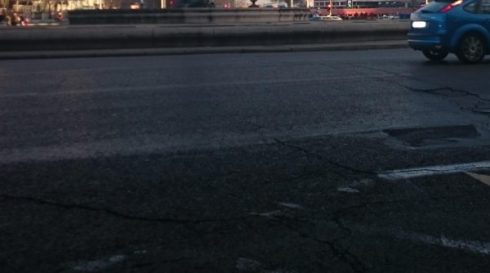
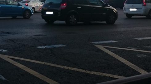
Here are the four cropped images:
print('Predicted:', decode_predictions(pred, top=3)[0])
Predicted: [('n03770679', 'minivan', 0.12950829), ('n02930766', 'cab', 0.113266684), ('n04461696', 'tow_truck', 0.09845059)]
I decided to re-run cropped image 4 through the classifier (the one with the cars present).
We see that the classifier detects the presence of a vehicle in the image (probabilities appear for the terms ‘minivan’, ‘cab’, and ‘tow_truck’). While the probabilities themselves are quite low, the model has correctly identified the general category of the object in the image, i.e. a vehicle, and is therefore considered suitable for this purpose. For instance, an autonomous car needs to detect the presence of a vehicle on the road first and foremost, rather than necessarily classifying that vehicle as a cab or a minivan.
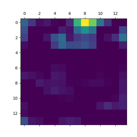
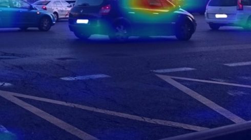
Here are the heatmaps for the cropped image:
We now see that the focus is on the car for the cropped image.
Analysis for Stockholm
The same VGG16 model was generated for Stockholm, and these were the results and heatmap:
print('Predicted:', decode_predictions(pred, top=3)[0])
Predicted: [('n03877845', 'palace', 0.7787534), ('n04335435', 'streetcar', 0.151575), ('n04486054', 'triumphal_arch', 0.013562491)]
As we can see, the zone in the heatmap is focused around the building rather than the vehicles, with the classifier identifying the building in question as a ‘palace’.
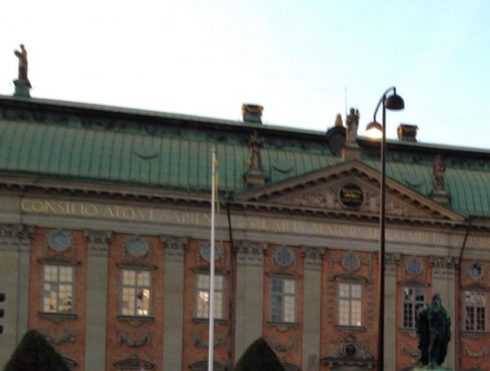
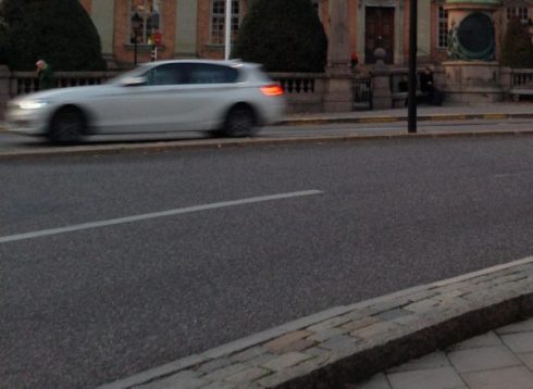
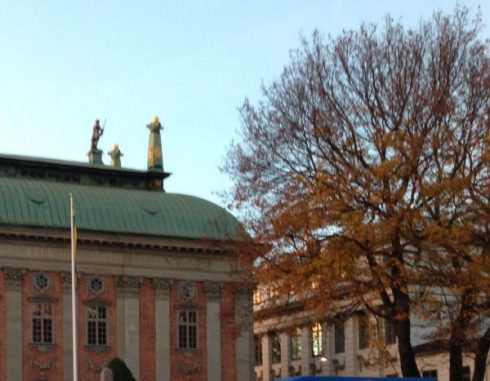
Again, it was decided to crop the image into four separate quadrants:
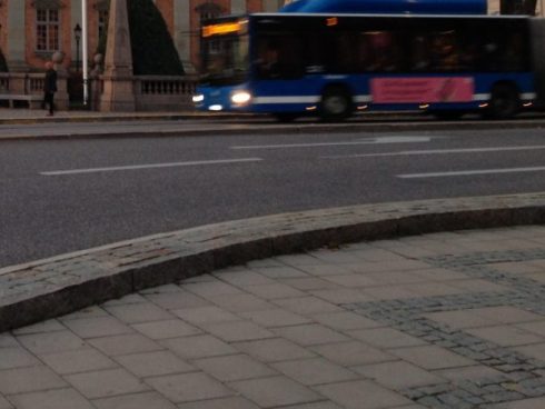
Let’s take the example of image 4 – the image of the bus.
Upon running the classifier, the following results were obtained:
print('Predicted:', decode_predictions(pred, top=3)[0])
Predicted: [('n04335435', 'streetcar', 0.59897834), ('n04487081', 'trolleybus', 0.072266325), ('n06874185', 'traffic_light', 0.065069936)]
The following predictions are generated: ‘streetcar’, ‘trolleybus’, and ‘traffic_light’. The classifier identifies that the vehicle is a larger one, and we can see that this is possible when we take the image of the bus in isolation.
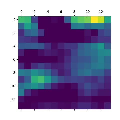
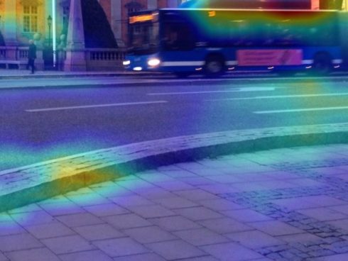
Here is the heatmap for the cropped image:
Again, the focus is now on the bus in the heatmap for the cropped image.
Video Frame Extraction with OpenCV
Having looked at how to classify images with VGG16, how would this scenario play out in the context of autonomous driving? It is important to remember that in many contexts, images are not being classified in isolation.
Rather, frames are being extracted from video, which are then analysed with a neural network. The way this can be done is by using the OpenCV library.
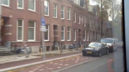
Let’s take this 10-second video as an example. Here, a bus is driving through a busy street in Amsterdam, and the purpose of the classifier is to identify the road objects within the frames.
To split the video into different frames, i.e. extract all the images from the video, OpenCV can be used as follows:
import cv2
print(cv2.__version__)
vidcap = cv2.VideoCapture('filepath/amsterdam.mp4')
success,image = vidcap.read()
count = 0
success = True
while success:
  cv2.imwrite("frame%d.jpg" % count, image)     # save frame as JPEG file
  success,image = vidcap.read()
  print ('Read a new frame: ', success)
  count += 1
This particular video is split into 302 different frames. Let’s use frame 216 as an example.
As before, the frame is cropped into four separate quadrants:
from PIL import Image
baseheight = 700
img = Image.open('frame216.jpg')
hpercent = (baseheight / float(img.size[1]))
width = int((float(img.size[0]) * float(hpercent)))
img = img.resize((width, baseheight), Image.ANTIALIAS)
img.save('resizedimageframe216.jpg')

h1=baseheight/2
w1=width/2

croppedIm = img.crop((0, 0, w1, h1)) # left, up, right, bottom
croppedIm.save('croppedframe1.jpg')

croppedIm = img.crop((0, h1, w1, baseheight)) # left, up, right, bottom
croppedIm.save('croppedframe2.jpg')

croppedIm = img.crop((w1, 0, width, h1)) # left, up, right, bottom
croppedIm.save('croppedframe3.jpg')

croppedIm = img.crop((w1, h1, width, baseheight)) # left, up, right, bottom
croppedIm.save('croppedframe4.jpg')
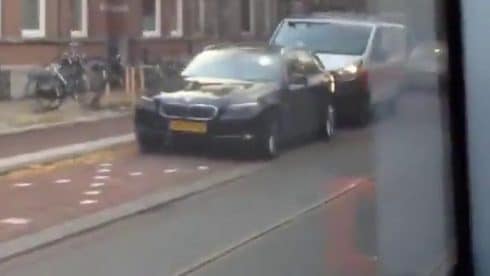
Let’s take the fourth quadrant for analysis.
Again, the classifier is run and the heatmaps are generated:
# Import Libraries
from keras.preprocessing.image import load_img
from keras.preprocessing.image import img_to_array
from keras.applications.vgg16 import preprocess_input
from keras.applications.vgg16 import decode_predictions
from keras.applications.vgg16 import VGG16
from keras import backend as K
import matplotlib.pyplot as plt
import numpy as np

# Process Model
model = VGG16()
image = load_img('croppedframe4.jpg', target_size=(224, 224))
image = img_to_array(image)
image = image.reshape((1, image.shape[0], image.shape[1], image.shape[2]))
image = preprocess_input(image)

# Generate predictions
pred = model.predict(image)
print('Predicted:', decode_predictions(pred, top=10)[0])
np.argmax(pred[0])

# Grad-CAM algorithm
specoutput=model.output[:, 803]
last_conv_layer = model.get_layer('block5_conv3')
grads = K.gradients(specoutput, last_conv_layer.output)[0]
pooled_grads = K.mean(grads, axis=(0, 1, 2))
iterate = K.function([model.input], [pooled_grads, last_conv_layer.output[0]])
pooled_grads_value, conv_layer_output_value = iterate([image])
for i in range(512):
    conv_layer_output_value[:, :, i] *= pooled_grads_value[i]

heatmap=np.mean(conv_layer_output_value, axis=-1)

# Heatmap post processing
heatmap = np.maximum(heatmap, 0)
heatmap /= np.max(heatmap)
plt.matshow(heatmap)
plt.show()

# Superimposing heatmap
import cv2
img = cv2.imread('croppedframe4.jpg')
heatmap = cv2.resize(heatmap, (img.shape[1], img.shape[0]))
heatmap = np.uint8(255 * heatmap)
heatmap = cv2.applyColorMap(heatmap, cv2.COLORMAP_JET)
superimposed_img = heatmap * 0.4 + img
cv2.imwrite('heatmaps1.jpg', superimposed_img)
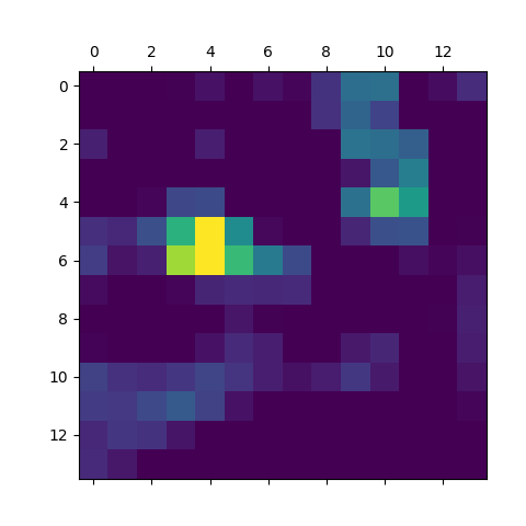
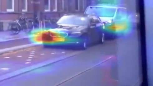
Here are the heatmaps and superimposed heatmaps:
And, here are the top 10 predictions:
print('Predicted:', decode_predictions(pred, top=10)[0])
Predicted: [('n04252225', 'snowplow', 0.1072438), ('n04467665', 'trailer_truck', 0.09812829), ('n03796401', 'moving_van', 0.07328106), ('n03384352', 'forklift', 0.054571714), ('n04487081', 'trolleybus', 0.05087295), ('n03417042', 'garbage_truck', 0.047520507), ('n04335435', 'streetcar', 0.045867864), ('n02965783', 'car_mirror', 0.02967672), ('n04461696', 'tow_truck', 0.02959971), ('n03345487', 'fire_engine', 0.026336407)]
As in previous classifications, the probability for each term is not overwhelmingly high, but the classifier does identify “streetcar” and “moving van” as potential classifications, which comes quite close to what we observe in the cropped image. Again, if we are looking for a classifier to identify the presence of a vehicle in the road – regardless of the probability attached to that classification – then this classifier would fit the bill.
Conclusion
In this example, you have seen:
- How to use VGG16 to construct an image classifier
- Generation of heatmaps with the cv2 library for determining classification “zones” in the image
- How to crop images with PIL to aid more accurate classification
- Use of OpenCV in extracting video frames
Many thanks for your time, and please feel free to leave any questions or comments below.
