We have previously added a set of company identity-agnostic predictors, such as the number of drivers a company employs, or the number of vehicles in the fleet with a hydraulic lift, and so on. we took this approach, rather than having each company as a unique predictor, so that the addition of a new contractor would not (necessarily) confuse our model.
I understand that this means company history, specific vehicle history, and so on, are not included. Nevertheless, we want to see how much information is in the new predictors.
Data exploration
in_csv <- "../output/intermediate/ii_times.csv"
ii_times <- read_csv(in_csv) %>%
  filter(reported_before_resolved == 1) %>% #we kept these flags for exploration, but they are troublesome for our real prediction. If we know a case has already been resolved, our model looks better than it is at predicting delays.
  mutate(reported_before_resolved = NULL)

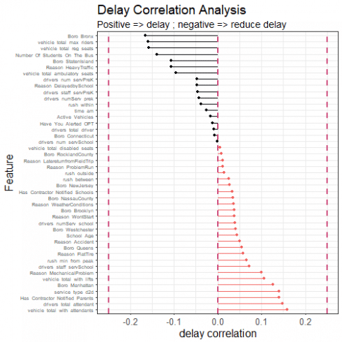
#first we look at the correlation of the predictors with the time_delayed:
corrr_analysis <- ii_times %>%
  select(-Busbreakdown_ID) %>%
  correlate() %>%
  focus(time_delayed) %>%
  rename(feature = rowname) %>%
  arrange(desc(abs(time_delayed))) %>%
  mutate(feature = as_factor(feature))
corrr_analysis %>% print(n=61)
## # A tibble: 45 x 2
##    feature                         time_delayed
##    <fct>                                  <dbl>
##  1 Boro_Bronx                          -0.166
##  2 vehicle_total_max_riders            -0.159
##  3 vehicle_total_with_attendants        0.159
##  4 vehicle_total_reg_seats             -0.157
##  5 drivers_total_attendant              0.147
##  6 Has_Contractor_Notified_Parents      0.140
##  7 service_type_d2d                     0.140
##  8 Number_Of_Students_On_The_Bus       -0.139
##  9 Boro_Manhattan                       0.125
## 10 Boro_StatenIsland                   -0.106
## 11 Reason_HeavyTraffic                 -0.106
## 12 vehicle_total_with_lifts             0.106
## 13 Reason_MechanicalProblem             0.100
## 14 vehicle_total_ambulatory_seats      -0.0960
## 15 drivers_staff_servSchool             0.0716
## 16 rush_min_from_peak                   0.0648
## 17 Reason_FlatTire                      0.0582
## 18 Boro_Queens                          0.0550
## 19 Reason_Accident                      0.0503
## 20 drivers_num_servPreK                -0.0478
## 21 Reason_DelayedbySchool              -0.0471
## 22 drivers_staff_servPreK              -0.0468
## 23 School_Age                           0.0441
## 24 drivers_numServ_prek                -0.0425
## 25 Boro_Westchester                     0.0400
## 26 drivers_numServ_school               0.0390
## 27 rush_within                         -0.0385
## 28 Reason_WontStart                     0.0383
## 29 Boro_Brooklyn                        0.0378
## 30 Reason_WeatherConditions             0.0367
## 31 Boro_NassauCounty                    0.0345
## 32 Has_Contractor_Notified_Schools      0.0334
## 33 Boro_NewJersey                       0.0265
## 34 time_am                             -0.0257
## 35 rush_between                         0.0254
## 36 Active_Vehicles                     -0.0164
## 37 rush_outside                         0.0152
## 38 Reason_ProblemRun                    0.0115
## 39 Have_You_Alerted_OPT                -0.0113
## 40 Reason_LatereturnfromFieldTrip       0.0109
## 41 drivers_total_driver                -0.00878
## 42 Boro_RocklandCounty                  0.00809
## 43 Boro_Connecticut                    -0.00787
## 44 vehicle_total_disabled_seats         0.00572
## 45 drivers_num_servSchool              -0.00182
#NR: there are some NAs here. I need to have a look at them. These are the no-information columns.

corrr_analysis %>%
  filter(!is.na(time_delayed)) %>%
  ggplot(aes(x = time_delayed, y = fct_reorder(feature, desc(time_delayed)))) +
  geom_point() +
  # Positive Correlations - Contribute to churn
  geom_segment(aes(xend = 0, yend = feature),
    color = magma(4)[[3]],
    data = corrr_analysis %>% filter(time_delayed > 0)) +
  geom_point(color = magma(4)[[3]],
    data = corrr_analysis %>% filter(time_delayed > 0)) +
  # Negative Correlations - Prevent churn
  geom_segment(aes(xend = 0, yend = feature),
    color = magma(4)[[1]],
    data = corrr_analysis %>% filter(time_delayed < 0)) +
  geom_point(color = magma(4)[[1]],
    data = corrr_analysis %>% filter(time_delayed < 0)) +
  # Vertical lines
  geom_vline(xintercept = 0, color = plasma(3)[[2]], size = 1, linetype = 2) +
  geom_vline(xintercept = -0.25, color = plasma(3)[[2]], size = 1, linetype = 2) +
  geom_vline(xintercept = 0.25, color = plasma(3)[[2]], size = 1, linetype = 2) +
  # Aesthetics
  theme_bw() +
  labs(title = "Delay Correlation Analysis",
    subtitle = paste("Positive => delay",
      "; negative => reduce delay"),
    x = "delay correlation", y = "Feature") +
  theme(text=element_text(family="Arial", size=16), axis.text.y = element_text(size=7))
There are already some interesting insights from these data. Drivers appear more likely to alert OPT for delays which end up shorter. Companies with a lot of ambulatory seats in their fleet suffer shorter delays. Services closer to peak hour suffer lower delays, something of a surprise. Companies with a lot of attendants and hydraulic lifts suffer longer delays. Having a high number of pre-K services disposes a company towards less delay; having a high number of school services disposes them towards more delay. And so on. We also see that there is structure from the original data, including different delays for different boroughs, and for different reasons.
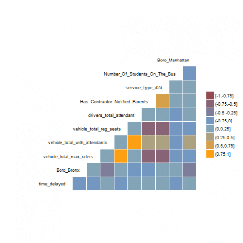
One of the first questions we might ask of all these predictors is: are they correlated with each other? If they are not, then perhaps we could, at some stage, run a naive Bayesian classification. Let's take a look at the cross-correlations between some of the predictors. We include 'time_delayed' for reference:
corrr_high <- corrr_analysis %>%
  mutate(feature = as.character(feature)) %>%
  filter(feature != "reported_before_resolved") %>%
  filter(abs(time_delayed) >= quantile(abs(corrr_analysis$time_delayed), 0.8) ) %>%
  dplyr::select(feature) %>%
  as.data.frame()


ii_times %>%
  select(time_delayed, corrr_high[[1]]) %>%
  ggcorr(nbreaks = 8, low = "#924A51", mid = "#70A5D4", high = "#FE9F14",
    max_size = 20,
    min_size = 2,
    size = 3,
    hjust = 1,
    vjust = 0.5,
    angle = 0,
    layout.exp = 4)
Even in this reduced set of 'more important' predictors, we can see that many predictors correlate more strongly with each other than with the target variable (time_delayed). This seems pretty bad news for the independence assumption of naive Bayes. The data set also might be a candidate for dimensionality reduction, but at this stage I wanted to keep things as human-transparent as possible.
Building a Cubist regression model with the extra predictors
This next part is straightforward. We go through essentially the same process that we did before, but this time we are armed with the extra predictors. If these predictors are useful, our RMSE should be lower and our \(R^2\) should be higher.
halfFold <- createFolds(ii_times$time_delayed, k = 5, list=TRUE)
ii_small <- ii_times[halfFold[[2]],]
ii_test <-ii_times[halfFold[[3]],]
ii_train <- ii_times %>%
  anti_join(ii_test, by = "Busbreakdown_ID")
rctrl_manual <- trainControl(method = "none", returnResamp = "all")
rctrl_repcv <- trainControl(method = "repeatedcv", number = 2, repeats = 5, returnResamp = "all")
#---There is actually a problem here. If I do not use the reported_before_resolved flag, I should remove those points from the data set. Do this and retry.
#---cubist
cubist_grd <- expand.grid(
  committees = 75,
  neighbors = 0
)
set.seed(849)
cubist_cv <- train(time_delayed ~ . -Busbreakdown_ID,
  data = ii_small,
  method = "cubist",
  metric="RMSE",
  na.action = na.pass,
  trControl = rctrl_repcv,
  tuneGrid = cubist_grd,
  control = Cubist::cubistControl(unbiased = T, rules = 30, sample = 0)
)
cubist_cv
## Cubist
##
## 40665 samples
##    46 predictor
##
## No pre-processing
## Resampling: Cross-Validated (2 fold, repeated 5 times)
## Summary of sample sizes: 20333, 20332, 20333, 20332, 20331, 20334, ...
## Resampling results:
##
##   RMSE      Rsquared   MAE
##   11.74162  0.3502251  8.273603
##
## Tuning parameter 'committees' was held constant at a value of 75
##
## Tuning parameter 'neighbors' was held constant at a value of 0
#comm75, rules30: 0.355, RMSE 11.72
cubist_cv$finalModel$splits %>% glimpse
## Observations: 8,341
## Variables: 8
## $ committee  <dbl> 1, 1, 1, 1, 1, 1, 1, 1, 1, 1, 1, 1, 1, 1, 1, 1, 1, ...
## $ rule       <dbl> 1, 1, 1, 1, 2, 2, 2, 3, 3, 3, 3, 3, 4, 4, 4, 4, 4, ...
## $ variable   <fct> Number_Of_Students_On_The_Bus, vehicle_total_with_l...
## $ dir        <fct> >, <=, <=, <=, >, <=, >, >, >, <=, >, <=, >, <=, >,...
## $ value      <dbl> 4, 4, 225, 5449, 0, 389, 601, 7, 131, 5449, 4, 82, ...
## $ category   <fct> , , , , , , , , , , , , , , , , , , , , , , , ,
## $ type       <chr> "type2", "type2", "type2", "type2", "type2", "type2...
## $ percentile <dbl> 0.8056068, 0.3884421, 0.4687077, 0.5004795, 0.94132...
cubist_cv$finalModel$coefficients %>% glimpse
## Observations: 2,234
## Variables: 48
## $ `(Intercept)`                   <dbl> 26.4, 59.3, 11.1, 19.1, 17.7, ...
## $ Has_Contractor_Notified_Schools <dbl> NA, 1.5, NA, 0.7, NA, NA, 3.3,...
## $ Has_Contractor_Notified_Parents <dbl> 0.6, 1.3, 1.5, 0.5, NA, 2.5, N...
## $ Have_You_Alerted_OPT            <dbl> 1.4, -0.6, -4.5, -2.4, 0.4, -1...
## $ Number_Of_Students_On_The_Bus   <dbl> -0.14, -0.07, -0.14, -0.08, -0...
## $ School_Age                      <dbl> NA, NA, NA, NA, NA, NA, NA, NA...
## $ Reason_Accident                 <dbl> 4, 6, NA, 2, NA, NA, NA, NA, 7...
## $ Reason_DelayedbySchool          <dbl> -2, NA, NA, NA, NA, NA, NA, NA...
## $ Reason_FlatTire                 <dbl> 2, 4, NA, NA, NA, NA, NA, NA, ...
## $ Reason_HeavyTraffic             <dbl> -2.4, -1.1, NA, -0.4, -3.7, NA...
## $ Reason_LatereturnfromFieldTrip  <dbl> NA, 1.1, NA, NA, NA, NA, NA, 1...
## $ Reason_MechanicalProblem        <dbl> 2.2, 2.5, NA, 0.8, NA, NA, NA,...
## $ Reason_ProblemRun               <dbl> NA, 2, NA, NA, NA, NA, NA, NA,...
## $ Reason_WeatherConditions        <dbl> NA, 3.9, NA, NA, 5.0, NA, NA, ...
## $ Reason_WontStart                <dbl> 2, 2, NA, NA, NA, NA, NA, NA, ...
## $ Boro_Bronx                      <dbl> 0.6, 0.6, -1.1, -1.3, 4.2, -2....
## $ Boro_Brooklyn                   <dbl> 2.4, -0.4, NA, 2.5, 0.6, 1.4, ...
## $ Boro_Connecticut                <dbl> NA, NA, NA, NA, NA, NA, NA, NA...
## $ Boro_Manhattan                  <dbl> 2.3, 1.5, -1.0, -0.4, 0.6, NA,...
## $ Boro_NassauCounty               <dbl> 4, 2, NA, NA, NA, NA, NA, NA, ...
## $ Boro_NewJersey                  <dbl> NA, NA, NA, NA, NA, NA, NA, NA...
## $ Boro_Queens                     <dbl> 3.9, 0.7, NA, NA, 0.8, NA, -4....
## $ Boro_RocklandCounty             <dbl> NA, NA, NA, NA, NA, NA, NA, NA...
## $ Boro_StatenIsland               <dbl> NA, 1.9, NA, NA, NA, NA, NA, N...
## $ Boro_Westchester                <dbl> 2.5, NA, NA, NA, NA, NA, NA, N...
## $ drivers_numServ_school          <dbl> -2.0, NA, NA, NA, -0.3, NA, NA...
## $ drivers_numServ_prek            <dbl> -2.4, NA, NA, NA, NA, NA, NA, ...
## $ drivers_total_driver            <dbl> 0.0330, -0.4627, 0.1162, 0.523...
## $ drivers_total_attendant         <dbl> -0.1228, -0.4552, 0.2071, 0.29...
## $ drivers_num_servPreK            <dbl> -0.592, NA, -0.463, -0.872, -0...
## $ drivers_num_servSchool          <dbl> NA, NA, NA, NA, -1.7894, NA, 1...
## $ drivers_staff_servPreK          <dbl> 0.303, NA, NA, NA, -0.982, 0.0...
## $ drivers_staff_servSchool        <dbl> 0.0372, 0.3984, -0.2191, -0.42...
## $ Active_Vehicles                 <dbl> 0.4074, 0.0722, 0.0733, 0.1984...
## $ vehicle_total_max_riders        <dbl> -0.00330, 0.00047, 0.02326, 0....
## $ vehicle_total_reg_seats         <dbl> -0.00571, -0.00160, -0.01979, ...
## $ vehicle_total_disabled_seats    <dbl> NA, -0.0183, -0.0368, -0.0802,...
## $ vehicle_total_ambulatory_seats  <dbl> NA, NA, NA, NA, NA, NA, NA, 0....
## $ vehicle_total_with_lifts        <dbl> 14.131, 0.130, 0.120, 0.460, 1...
## $ vehicle_total_with_attendants   <dbl> -0.2296, -0.0095, -0.0022, -0....
## $ service_type_d2d                <dbl> -1.6, 0.5, NA, -1.8, -0.6, -0....
## $ time_am                         <dbl> -5.0, -0.5, NA, NA, NA, NA, 4....
## $ rush_within                     <dbl> -2.3, 1.3, NA, NA, -1.3, -2.8,...
## $ rush_between                    <dbl> -4.8, -1.2, NA, -1.3, -3.2, -5...
## $ rush_outside                    <dbl> -1.6, 0.6, NA, -0.4, -3.5, -2....
## $ rush_min_from_peak              <dbl> NA, 0.019, NA, 0.006, NA, 0.02...
## $ committee                       <chr> "1", "1", "1", "1", "1", "1", ...
## $ rule                            <chr> "1", "2", "3", "4", "5", "6", ...
cubist_cv$finalModel$usage %>% head
##   Conditions Model                       Variable
## 1         48    86        vehicle_total_reg_seats
## 2         41    20 vehicle_total_ambulatory_seats
## 3         37    75       vehicle_total_with_lifts
## 4         35    49            Reason_HeavyTraffic
## 5         28    90       vehicle_total_max_riders
## 6         24    86  vehicle_total_with_attendants
cubist_man <- train(time_delayed ~ . -Busbreakdown_ID,
  data = ii_train,
  method = "cubist",
  metric="RMSE",
  na.action = na.pass,
  trControl = rctrl_manual,
  tuneGrid = cubist_grd,
  control = Cubist::cubistControl(unbiased = T, rules = 30, sample = 0)
)
ii_withpred <- ii_test %>%
  mutate(
    time_predicted = predict(cubist_man, newdata = ii_test)
  )
ii_withpred %>%
  summarise(
    rms = (mean((time_predicted-time_delayed)^2))^0.5,
    sum_sq = sum((time_predicted-time_delayed)^2),
    tot_sum_sq = sum((time_delayed - mean(time_delayed))^2),
    r_sq = 1- sum_sq / tot_sum_sq
  ) #0.371, RMSE 11.6
## # A tibble: 1 x 4
##     rms   sum_sq tot_sum_sq  r_sq
##   <dbl>    <dbl>      <dbl> <dbl>
## 1  11.5 5422077.   8556551. 0.366
ii_overfit <- ii_train %>%
  mutate(
    time_predicted = predict(cubist_man, newdata = ii_train)
  )
ii_overfit %>%
  summarise(
    rms = (mean((time_predicted-time_delayed)^2))^0.5,
    sum_sq = sum((time_predicted-time_delayed)^2),
    tot_sum_sq = sum((time_delayed - mean(time_delayed))^2),
    r_sq = 1- sum_sq / tot_sum_sq
  ) #0.374, RMSE 11.5: the overfit is not too bad.
## # A tibble: 1 x 4
##     rms    sum_sq tot_sum_sq  r_sq
##   <dbl>     <dbl>      <dbl> <dbl>
## 1  11.5 21412743.  34357934. 0.377
protec <- ii_withpred %>%
  mutate(Reason_Other = 1L) %>% #dummy flag to get the name in
  select(-contains("Reason")) %>%
  colnames()
pal <- brewer.pal(10, "Paired")
ii_withpred %>%
  mutate(Reason_Other = ifelse(Reason_Accident + Reason_DelayedbySchool + Reason_FlatTire + Reason_HeavyTraffic + Reason_LatereturnfromFieldTrip + Reason_MechanicalProblem + Reason_ProblemRun + Reason_WeatherConditions + Reason_WontStart == 1, 0L, 1L)) %>%
  gather(key = Reason, value = dummy, -one_of(protec)) %>%
  filter(dummy == 1) %>%
  mutate(dummy = NULL) %>%
  filter(row_number() %% 10 == 0) %>%
  ggplot(aes(x = time_predicted, y = time_delayed, fill = Reason, color = Reason)) +
  geom_point(alpha = 0.75, shape = 21) +
  scale_fill_manual(values = pal) +
  geom_abline(intercept = 0, slope = 1, color = "red") +
  coord_cartesian(expand = c(0,0), x = c(0,60)) +
  theme_classic() +
  labs(x="time_predicted [min]",y="time_delayed [min]") +
  theme(text=element_text(family="Arial", size=16)) +
  theme(axis.line = element_line(colour = 'black', size = 1)) +
  theme(axis.ticks = element_line(colour = "black", size = 1)) +
  ggtitle("Cubist with extra predictors: delayed vs predicted")
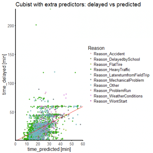
We have more than doubled our \(R^2\) value, although we are still below 0.5. Our time_delayed vs time_predicted is starting to cluster more around the line of perfect prediction. We are still mispredicting a lot of delay times, but we are certainly doing better than before.
While there is possibly more to be done to improve our predictors, we can guess that we might not get too much further with this approach. We know that our data have a problem related to how delays have been reported, and it isn't going to go away. So perhaps we ought to try the problem as a classification: how well can we predict if delay time will be above some arbitrary threshold? This is the approach we take next.


