I have been using keras and TensorFlow for a while now – and love its simplicity and straight-forward way to modeling. As part of the latest update to my workshop about deep learning with R and keras I've added a new example analysis such as Building an image classifier to differentiate different types of fruits.
And I was (again) surprised how fast and easy it was to build the model; it took not even half an hour and only around 100 lines of code (counting only the main code; for this post, I added comments and line breaks to make it easier to read)! That's why I wanted to share it here and spread the keras love.
The code
If you haven't installed keras before, follow the instructions of RStudio's keras site
library(keras)
The dataset is the fruit images dataset from Kaggle. I downloaded it to my computer and unpacked it. Because I don't want to build a model for all the different fruits, I define a list of fruits (corresponding to the folder names) that I want to include in the model.
I also define a few other parameters, in the beginning, to make adapting as easy as possible.
# list of fruits to modle
fruit_list <- c("Kiwi", "Banana", "Apricot", "Avocado", "Cocos", "Clementine", "Mandarine", "Orange",
                "Limes", "Lemon", "Peach", "Plum", "Raspberry", "Strawberry", "Pineapple", "Pomegranate")

# number of output classes (i.e. fruits)
output_n <- length(fruit_list)

# image size to scale down to (original images are 100 x 100 px)
img_width <- 20
img_height <- 20
target_size <- c(img_width, img_height)

# RGB = 3 channels
channels <- 3

# path to image folders
train_image_files_path <- "/Users/shiringlander/Documents/Github/DL_AI/Tutti_Frutti/fruits-360/Training/"
valid_image_files_path <- "/Users/shiringlander/Documents/Github/DL_AI/Tutti_Frutti/fruits-360/Validation/"
Loading images
The handy image_data_generator() and flow_images_from_directory() functions can be used to load images from a directory. If you want to use data augmentation, you can directly define how and in what way you want to augment your images with image_data_generator. Here I am not augmenting the data, I only scale the pixel values to fall between 0 and 1.
# optional data augmentation
train_data_gen = image_data_generator(
  rescale = 1/255 #,
  #rotation_range = 40,
  #width_shift_range = 0.2,
  #height_shift_range = 0.2,
  #shear_range = 0.2,
  #zoom_range = 0.2,
  #horizontal_flip = TRUE,
  #fill_mode = "nearest"
)

# Validation data shouldn't be augmented! But it should also be scaled.
valid_data_gen <- image_data_generator(
  rescale = 1/255
  )
Now we load the images into memory and resize them.
# training images
train_image_array_gen <- flow_images_from_directory(train_image_files_path,
                                          train_data_gen,
                                          target_size = target_size,
                                          class_mode = "categorical",
                                          classes = fruit_list,
                                          seed = 42)

# validation images
valid_image_array_gen <- flow_images_from_directory(valid_image_files_path,
                                          valid_data_gen,
                                          target_size = target_size,
                                          class_mode = "categorical",
                                          classes = fruit_list,
                                          seed = 42)
cat("Number of images per class:")
## Number of images per class:
table(factor(train_image_array_gen$classes))
##   0   1   2   3   4   5   6   7   8   9  10  11  12  13  14  15
## 466 490 492 427 490 490 490 479 490 492 492 447 490 492 490 492
cat("\nClass label vs index mapping:\n")
## Class label vs index mapping:
train_image_array_gen$class_indices
## $Lemon
## [1] 9
##
## $Peach
## [1] 10
##
## $Limes
## [1] 8
##
## $Apricot
## [1] 2
##
## $Plum
## [1] 11
##
## $Avocado
## [1] 3
##
## $Strawberry
## [1] 13
##
## $Pineapple
## [1] 14
##
## $Orange
## [1] 7
##
## $Mandarine
## [1] 6
##
## $Banana
## [1] 1
##
## $Clementine
## [1] 5
##
## $Kiwi
## [1] 0
##
## $Cocos
## [1] 4
##
## $Pomegranate
## [1] 15
##
## $Raspberry
## [1] 12
fruits_classes_indices <- train_image_array_gen$class_indices
save(fruits_classes_indices, file = "/Users/shiringlander/Documents/Github/DL_AI/Tutti_Frutti/fruits-360/fruits_classes_indices.RData")
Define model
Next, we define the keras model.
# number of training samples
train_samples <- train_image_array_gen$n
# number of validation samples
valid_samples <- valid_image_array_gen$n

# define batch size and number of epochs
batch_size <- 32
epochs <- 10
The model I am using here is a very simple sequential convolutional neural net with the following hidden layers: 2 convolutional layers, one pooling layer and one dense layer.
# initialise model
model <- keras_model_sequential()

# add layers
model %>%
  layer_conv_2d(filter = 32, kernel_size = c(3,3), padding = "same", input_shape = c(img_width, img_height, channels)) %>%
  layer_activation("relu") %>%

  # Second hidden layer
  layer_conv_2d(filter = 16, kernel_size = c(3,3), padding = "same") %>%
  layer_activation_leaky_relu(0.5) %>%
  layer_batch_normalization() %>%

  # Use max pooling
  layer_max_pooling_2d(pool_size = c(2,2)) %>%
  layer_dropout(0.25) %>%

  # Flatten max filtered output into feature vector
  # and feed into dense layer
  layer_flatten() %>%
  layer_dense(100) %>%
  layer_activation("relu") %>%
  layer_dropout(0.5) %>%

  # Outputs from dense layer are projected onto output layer
  layer_dense(output_n) %>%
  layer_activation("softmax")

# compile
model %>% compile(
  loss = "categorical_crossentropy",
  optimizer = optimizer_rmsprop(lr = 0.0001, decay = 1e-6),
  metrics = "accuracy"
)
Fit the model; because I used image_data_generator() and flow_images_from_directory() I am now also using the fit_generator() to run the training.
# fit
hist <- model %>% fit_generator(
  # training data
  train_image_array_gen,

  # epochs
  steps_per_epoch = as.integer(train_samples / batch_size),
  epochs = epochs,

  # validation data
  validation_data = valid_image_array_gen,
  validation_steps = as.integer(valid_samples / batch_size),

  # print progress
  verbose = 2,
  callbacks = list(
    # save best model after every epoch
    callback_model_checkpoint("/Users/shiringlander/Documents/Github/DL_AI/Tutti_Frutti/fruits-360/keras/fruits_checkpoints.h5", save_best_only = TRUE),
    # only needed for visualising with TensorBoard
    callback_tensorboard(log_dir = "/Users/shiringlander/Documents/Github/DL_AI/Tutti_Frutti/fruits-360/keras/logs")
  )
)
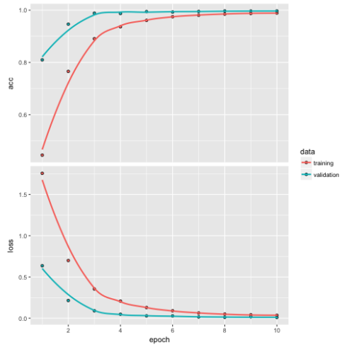
In RStudio we are seeing the output as an interactive plot in the “Viewer” pane but we can also plot it:
plot(hist)
As we can see, the model is quite accurate on the validation data. However, we need to keep in mind that our images are very uniform, they all have the same white background and show the fruits centered and without anything else in the images. Thus, our model will not work with images that don't look similar as the ones we trained on (that's also why we can achieve such good results with such a small neural net).
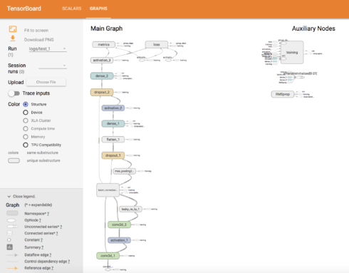
Finally, I want to have a look at the TensorFlow graph with TensorBoard.
tensorboard("/Users/shiringlander/Documents/Github/DL_AI/Tutti_Frutti/fruits-360/keras/logs")
That's all there is to it!
Of course, you could now save your model and/or the weights, visualize the hidden layers, run predictions on test data, etc. For now, I'll leave it at that, though.
sessionInfo()
## R version 3.5.0 (2018-04-23)
## Platform: x86_64-apple-darwin15.6.0 (64-bit)
## Running under: macOS High Sierra 10.13.5
##
## Matrix products: default
## BLAS: /System/Library/Frameworks/Accelerate.framework/Versions/A/Frameworks/vecLib.framework/Versions/A/libBLAS.dylib
## LAPACK: /Library/Frameworks/R.framework/Versions/3.5/Resources/lib/libRlapack.dylib
##
## locale:
## [1] de_DE.UTF-8/de_DE.UTF-8/de_DE.UTF-8/C/de_DE.UTF-8/de_DE.UTF-8
##
## attached base packages:
## [1] stats     graphics  grDevices utils     datasets  methods   base
##
## other attached packages:
## [1] keras_2.1.6      knitr_1.20       RWordPress_0.2-3
##
## loaded via a namespace (and not attached):
##  [1] Rcpp_0.12.17     highr_0.7        pillar_1.2.3     compiler_3.5.0
##  [5] plyr_1.8.4       bitops_1.0-6     base64enc_0.1-3  tools_3.5.0
##  [9] zeallot_0.1.0    digest_0.6.15    tibble_1.4.2     jsonlite_1.5
## [13] evaluate_0.10.1  gtable_0.2.0     lattice_0.20-35  rlang_0.2.1
## [17] Matrix_1.2-14    yaml_2.1.19      blogdown_0.6     xfun_0.2
## [21] stringr_1.3.1    rprojroot_1.3-2  grid_3.5.0       reticulate_1.8
## [25] R6_2.2.2         XML_3.98-1.11    rmarkdown_1.10   bookdown_0.7
## [29] reshape2_1.4.3   ggplot2_2.2.1    magrittr_1.5     whisker_0.3-2
## [33] backports_1.1.2  XMLRPC_0.3-0     scales_0.5.0     htmltools_0.3.6
## [37] tfruns_1.3       colorspace_1.3-2 labeling_0.3     tensorflow_1.8
## [41] stringi_1.2.3    RCurl_1.95-4.10  lazyeval_0.2.1   munsell_0.5.0

